Analysis of Algorithms: asymptotic notation and the Size of a Problem

Post Views: 95

In the vast universe of computer science, the design and analysis of algorithms play a crucial role in optimizing solutions to computational problems. To fully understand the efficiency and performance of an algorithm, it is essential to be able to evaluate how its behavior varies in relation to the size of the input problem. We will explore two fundamental concepts for the analysis of algorithms: asymptotic notation and problem size. These tools will allow us to address algorithm performance challenges in a clear and concise way.

[wpda_org_chart tree_id=43 theme_id=50]

Size of a Problem

The size of a problem in algorithms refers to the amount of resources required by an algorithm relative to the size of the input. Understanding how the size of the problem affects the performance of algorithms is critical to evaluating the efficiency of proposed solutions.

Example with Sorting:

Suppose we have a sorting algorithm. The size of the problem in this case could be the length of the array to sort. If the array has n elements, the size of the problem is n.

Influence on Performance:

The size of the problem is often related to the execution time and complexity of the algorithm. For example, an algorithm that sorts a small array may be efficient, but may become impractical when dealing with a very large array.

Growth Analysis:

Studying how the execution time of an algorithm grows in relation to the size of the problem is essential. Algorithms that maintain a constant running time as the problem grows (O(1)) are preferable to those that grow linearly (O(n)) or quadratically (O(n^2)).

Understanding Resources:

The size of the problem may also relate to resource usage, such as memory. Efficient algorithms should be able to handle large amounts of data without exhausting available resources.

Asymptotic Notation

problem approaches infinity. The three main asymptotic notations are:

O Big (O)
Omega (Ω)
Theta (Θ)

Big O notation describes the upper bound of an algorithm. In essence, it represents a way of expressing the worst case execution of an algorithm as a function of the size of the problem. For example, if an algorithm is $O(n^2)$ , it means that the running time grows quadratically with respect to the size of the problem.

Omega notation provides the lower bound of an algorithm, indicating the best possible case in terms of execution time. If an algorithm is Ω(n), it means that the running time grows at least linearly with the size of the problem.

Theta notation represents the average case of execution of an algorithm. If an algorithm is Θ(n), it means that the running time grows linearly with the size of the problem.

The Big O notation

First we give a formal definition of the notation.

Formal Definition of Big O Notation

Let $g(n)$ be a function of running time or space, and let $f(n)$ be the function associated with a particular algorithm.

The set $O(g(n))$ represents the set of all functions that grow at most as fast as a multiplicative constant of $g(n)$ for values sufficiently larger than $n$ . Formally, $f(n)$ is is $O(g(n)$ if there exist positive constants $c$ and $n_0$ such that for each $n \geq n_0$ , $f(n) \leq c \cdot g(n)$ .

In other words, Big O notation provides a way of describing the asymptotic behavior of a function, ignoring constant factors and less significant terms when considering sufficiently large inputs. It offers a way of characterizing the efficiency or complexity of an algorithm in a more general way.

Example:

Consider the function $f(n) = 3n^2 + 2n + 1$ and the function $g(n) = n^2$ . We will say that $f(n)$ is $O(n^2)$ if there exist positive constants $c$ and $n_0$ such that for each $n \geq n_0$ , $3n^2 + 2n + 1 \leq c \cdot n^2$ . In this case, we can choose $c = 6$ and $n_0 = 1$ , since for each $n \geq 1$ , $3n^2 + 2n + 1 \leq 6n^2$ .

Thus, the formal definition allows us to establish a mathematical link between functions and to express the growth of one function in relation to another.

Examples with Graphs in Python

O(1) – Constant execution time

import matplotlib.pyplot as plt
import numpy as np

def example_O_1():
    return 1

n_values = np.arange(1, 101)
time_complexity_values = [example_O_1() for _ in n_values]

plt.plot(n_values, time_complexity_values, label='O(1)')
plt.xlabel('n')
plt.ylabel('Execution time')
plt.title('O(1) - Constant time')
plt.legend()
plt.show()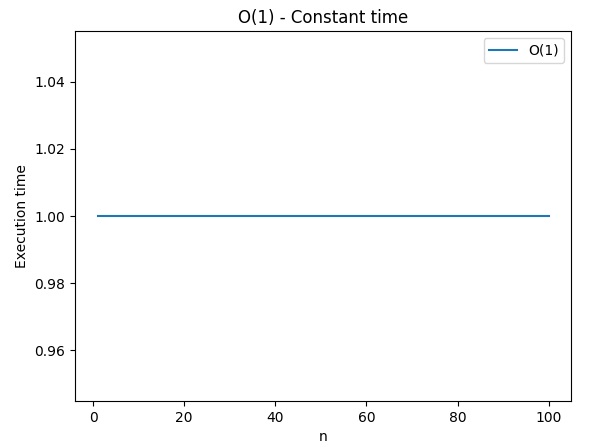

O(n) – Linear execution time

def example_O_n(n):
    return list(range(n))

plt.plot(n_values, [len(example_O_n(n)) for n in n_values], label='O(n)')
plt.xlabel('n')
plt.ylabel('Execution time')
plt.title('O(n) - Linear time')
plt.legend()
plt.show()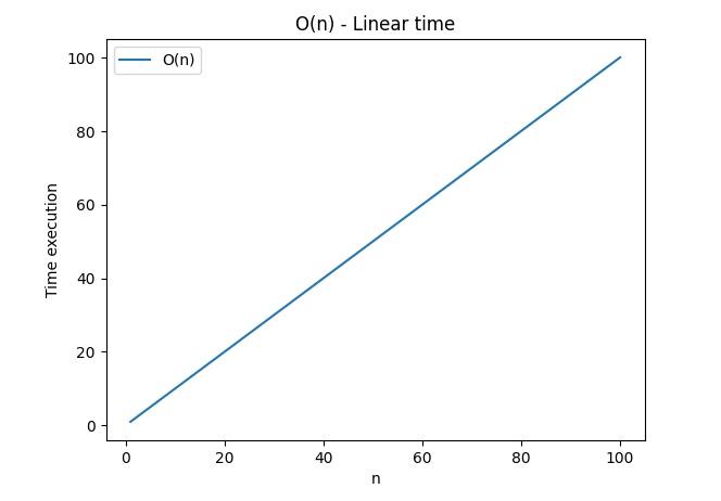

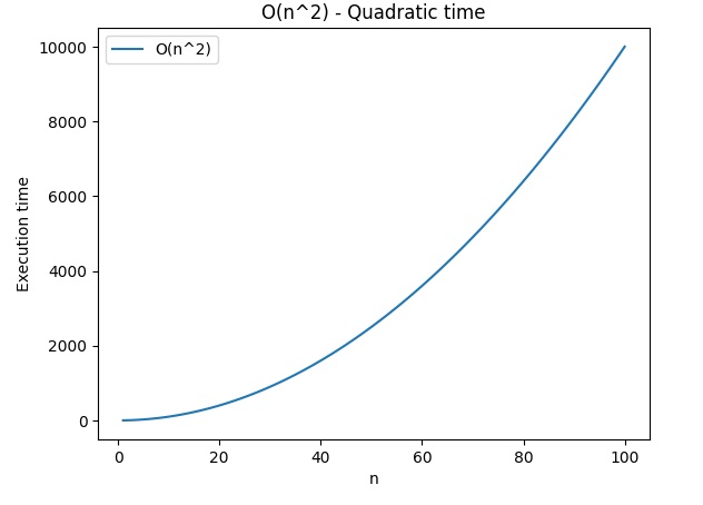
O(n^2) – Quadratic running time

def example_O_n_squared(n):
    result = []
    for i in range(n):
        for j in range(n):
            result.append((i, j))
    return result

# Plot del grafico
plt.plot(n_values, [len(example_O_n_squared(n)) for n in n_values], label='O(n^2)')
plt.xlabel('n')
plt.ylabel('Execution time')
plt.title('O(n^2) - Quadratic time')
plt.legend()
plt.show()

O(log n) – Logarithmic execution time

def example_O_log_n(n):
    return int(np.log2(n))

plt.plot(n_values, [example_O_log_n(n) for n in n_values], label='O(log n)')
plt.xlabel('n')
plt.ylabel('Execution time')
plt.title('O(log n) - Logaritmic time')
plt.legend()
plt.show()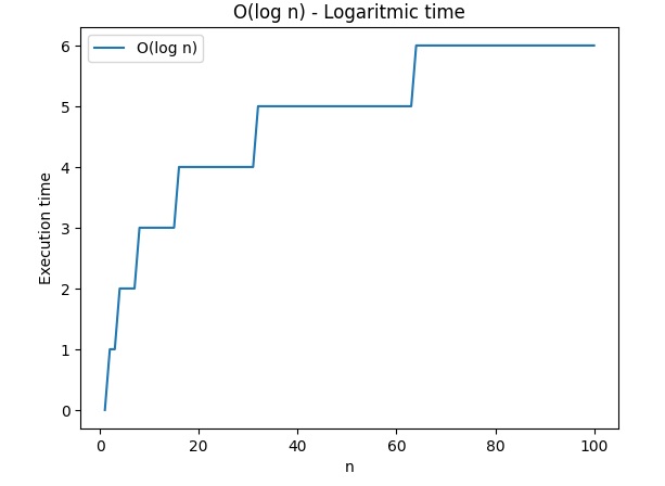

These examples graphically show how the execution time changes with respect to the size of the problem, following the different complexities indicated by the Big O notation.

Transition from problem size to asymptotic notation

Moving conceptually from the size of a problem to asymptotic notation involves analyzing the behavior of the algorithm as the size of the problem increases. Asymptotic notation provides a way of expressing the limiting behavior of an algorithm as the problem size approaches infinity.

Here’s how you can conceptually relate the size of a problem to asymptotic notation:

Observing Behavior: Start by observing how the running time or space required by the algorithm changes relative to the size of the problem. Ask yourself: Does it increase linearly, quadratically, logarithmically, or in some other way?
Identifying the Dominant Term: Identifies the dominant term that contributes most to the complexity of the algorithm. This term will be the basis of your asymptotic notation.
Match to Asymptotic Notation: Find the asymptotic notation that best describes the behavior of the algorithm. For example, if the dominant term is linear with respect to the problem size, you might use O(n) notation. If it is logarithmic, O(log n), and so on.
Consideration of Least Significant Terms: In asymptotic notation, what matters most is the dominant term. Less significant terms or multiplicative constants may be neglected. For example, if you have an algorithm with complexity 3n^2 + 5n + 7, the asymptotic notation will be O(n^2).
Checking the Properties of Asymptotic Notation: Make sure the asymptotic notation satisfies the fundamental properties. For example, O(n^2) indicates that the algorithm has quadratic behavior, but it does not imply anything about specific performance.

Let’s see a concrete example in Python of an algorithm with complexity (3n^2 + 5n + 7) and its comparison with (O(n^2)). We will create a graph to visualize the behavior of both trends.

import matplotlib.pyplot as plt
import numpy as np

# Algorithm with complexity 3n^2 + 5n + 7
def example_algorithm(n):
    return 3 * n**2 + 5 * n + 7

# Asymptotic notation O(n^2)
def o_notation(n):
    return n**2

# Size of the problem
n_values = np.arange(1, 101)

# Calculation of execution times
algorithm_values = [example_algorithm(n) for n in n_values]
o_notation_values = [o_notation(n) for n in n_values]

# Graph plot
plt.plot(n_values, algorithm_values, label='3n^2 + 5n + 7')
plt.plot(n_values, o_notation_values, label='O(n^2)')
plt.xlabel('Size of the Problem (n)')
plt.ylabel('Execution Time')
plt.title('Comparison between Algorithm and Asymptotic Notation')
plt.legend()
plt.show()

In this example, the algorithm is represented by the function (3n^2 + 5n + 7), while the asymptotic notation is represented by the function (O(n^2)). The graph shows how the execution time of the algorithm grows quadratically with respect to the size of the problem.

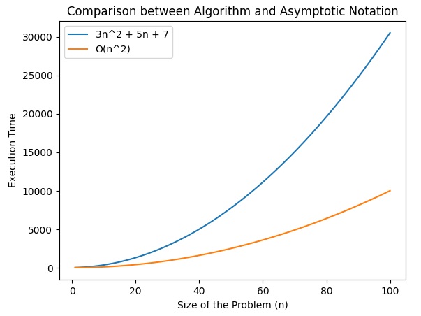
Why is (O(n^2)) considered:

In the term (3n^2 + 5n + 7), the dominant term driving the growth of the algorithm is (3n^2) (since it has a larger exponent than the others).
The asymptotic notation (O(n^2)) captures the overall behavior of the algorithm, focusing on the quadratic term as the problem size increases.
Least significant terms and multiplicative constants are neglected in asymptotic notation, focusing attention on the fundamental growth characteristics of the algorithm.

The graph shows how the execution time of the algorithm follows a quadratic trend, supporting the choice of (O(n^2)) as the appropriate asymptotic notation to describe the complexity of the algorithm.

Conclusion

In this article, we laid the foundation for algorithm analysis, introducing key concepts such as asymptotic notation and problem size. These too1s will help us clearly evaluate the performance of algorithms and design optimal solutions for a wide range of computational problems. In subsequent chapters, we will explore practical applications of these concepts, tackling concrete examples and deepening our understanding of the art and science behind algorithm design.