
Binary trees in Python are fundamental tools for organizing and managing data in a two-branch hierarchical structure. With Python, their implementation allows for easy manipulation of data, providing a solid foundation for operations such as inserting, searching, and removing.
[wpda_org_chart tree_id=43 theme_id=50]
Binary trees
A binary tree is a hierarchical data structure composed of nodes connected in such a way that each node can have at most two child nodes, called “left child” and “right child”. Every node, except the root, has exactly one parent node. The root is the main node of the tree, while nodes that have no children are called leaves.
- Node: Each element within the tree is called a node. Each node can have zero, one, or two child nodes, depending on its position in the tree.
- Root: The top node of the tree is the root. Every binary tree has only one root.
- Leaf: Nodes without child nodes are called leaves. They are the terminal nodes of the tree.
- Left and Right Child: Each node can have a maximum of two children, one on the left and one on the right. The left child is the child node positioned on the left side, while the right child is the one positioned on the right side.
Here are some important features that characterize binary trees
- Sorting: In some binary trees, such as binary search trees (BST), a sorting property is maintained, where nodes to the left of a given node contain lower values, while those to the right contain higher values.
- Recursive Structure: The structure of a binary tree is recursive, since each subtree of a node is also a binary tree.
Binary trees are used extensively in computer science to solve a variety of problems. Some common uses include representing mathematical expressions, creating binary search trees for efficient data searching, and structuring data in compilers.
In Python, binary trees can be implemented across classes and objects, taking advantage of the flexibility and clarity of the language to manage relationships between nodes efficiently and intuitively.
Compared to Graphs, Binary Trees are a specific type of acyclic (cycle-free) graph in which each node has at most two child nodes. Graphs can have an arbitrary number of connections between nodes. Binary trees are often used to represent ordered hierarchies, while graphs are more flexible and can represent more complex relationships.
In summary, binary trees provide an efficient data structure for representing hierarchical relationships and are particularly useful when you need to perform search operations or organize data in a way that reflects the logical relationships between them.
Types of Binary Trees
There are different types of binary trees, each of which has specific characteristics suitable for different contexts and implementation needs. Below, I present some of the main types of binary trees:
- Standard Binary Tree: Each node has at most two children: a left child and a right child.
- Binary Search Tree (BST): Binary tree structure in which each node has at most two children, and the value of the node on the left is less than or equal to the value of the parent node, while the value of the node on the right is greater.
- Complete Binary Tree: A binary tree in which all levels are completely filled, except possibly the last level which is filled from left to right.
- Perfect Binary Tree: A complete binary tree in which all levels are completely filled, thus having all leaves at the same level.
- Balanced Binary Tree: A binary tree in which the difference between the heights of the left and right subtrees of each node is at most one. AVL trees are an example of balanced binary trees.
- Binary Expression Tree: A binary tree used to represent mathematical expressions, where the operators are in the internal nodes and the operands are in the leaves.
- Huffman Tree: A type of binary tree used for data compression, in which more frequent characters have a shorter path than less frequent ones.
- Segment Tree: A binary tree used in range query algorithms that divides an array into segments and allows efficient operations to be performed on those ranges.
- Trie Tree (or Binary Trie): A type of binary tree in which each node represents a bit of a binary number and each path from the root to a leaf represents a unique binary number.
- Red-Black Tree: A type of binary search tree in which each node has a color attribute (red or black) and specific rules are applied to ensure approximate balancing of the tree.
Each type of binary tree has specific applications and advantages in terms of execution time of search, insertion and deletion operations. The choice of tree type depends on the specific needs of the problem you are addressing.
Python implementation of Binary Trees
To implement a binary tree in Python, you can use classes to represent the nodes and the tree itself. Here is an example implementation of a binary search tree (BST) in Python:
class Node:
    def __init__(self, value):
        self.value = value
        self.left_child = None
        self.right_child = None

    def __repr__(self):
        return f"Node with value {self.value}"

class BinarySearchTree:
    def __init__(self):
        self.root = None

    def insert(self, value):
        self.root = self._insert(self.root, value)

    def _insert(self, root, value):
        if root is None:
            return Node(value)

        if value < root.value:
            root.left_child = self._insert(root.left_child, value)
        elif value > root.value:
            root.right_child = self._insert(root.right_child, value)

        return root

    def search(self, value):
        return self._search(self.root, value)

    def _search(self, root, value):
        if root is None or root.value == value:
            return root
        if value < root.value:
            return self._search(root.left_child, value)
        return self._search(root.right_child, value)

    def in_order_traversal(self):
        result = []
        self._in_order_traversal(self.root, result)
        return result

    def _in_order_traversal(self, root, result):
        if root:
            self._in_order_traversal(root.left_child, result)
            result.append(root.value)
            self._in_order_traversal(root.right_child, result)

# Example usage:
tree = BinarySearchTree()
tree.insert(5)
tree.insert(3)
tree.insert(7)
tree.insert(1)
tree.insert(4)

print(tree.in_order_traversal())
print(tree.search(4))
print(tree.search(6))
In this example, we have a Node class that represents a single tree node and a BinarySearchTree class that represents the binary search tree. The tree is implemented with insert and search operations. In-order traversal is used to obtain an ordered list of the elements in the tree. Running the code you get the following result:
[1, 3, 4, 5, 7]
Node with value 4
None
This is just a basic example, and implementations may vary based on the specific needs of your project.
Visualizing Binary Trees with Graphviz
Graphviz è un insieme di strumenti open source per la visualizzazione di grafici. Consente di descrivere la struttura di un grafo attraverso un linguaggio di descrizione e di generare visualizzazioni grafiche del grafo in vari formati, come immagini PNG, PDF o SVG. Graphviz è ampiamente utilizzato per visualizzare la struttura di alberi, grafi, reti, schemi concettuali e altro ancora.
Il componente chiave di Graphviz è dot, un programma da riga di comando che legge la descrizione di un grafo e produce un file contenente la sua rappresentazione visiva.
- Install Graphviz: Make sure Graphviz is installed on your system. You can download it from Graphviz Download.
- Add Graphviz to the PATH: After installation, ensure that the path (PATH) to the Graphviz dot executable is added to your system’s environment variables.
- Check your Graphviz Installation: Verify that Graphviz is properly installed by running the dot command from a terminal window or command prompt. You should see a list of usage options.
Python module for Graphviz:
To interact with Graphviz through Python, you can use the graphviz module. This module provides a Python interface to generate Graphviz-compatible graph description files and to render these files to various image formats.
To install the graphviz module, you can use the following command:
pip install graphvizAfter installation, you can use the Python module in your code to generate graph descriptions and visualizations. Using the Graphviz module in Python is what we did in the previous example code to display the binary tree.
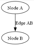
from graphviz import Digraph

# Creating a Digraph object
dot = Digraph(comment='GraphName')

# Adding nodes and arcs
dot.node('A', 'Node A')
dot.node('B', 'Node B')
dot.edge('A', 'B', label='Edge AB')

# Saving the graph in a file and rendering in a specific format (e.g. PNG)
dot.render('GraphName', format='png', cleanup=True)
This code creates a directed graph (Digraph), adds some nodes and an edge, and then renders the graph in PNG format. The resulting file can be viewed as an image or embedded in a Jupyter Notebook.
Let’s modify the previous example
Let’s make some changes to the example program used previously by integrating Graphviz.
from graphviz import Digraph
class Node:
def __init__(self, value):
self.value = value
self.left_child = None
self.right_child = None
def __repr__(self):
return f"Node with value {self.value}"
class BinarySearchTree:
def __init__(self):
self.root = None
def insert(self, value):
self.root = self._insert(self.root, value)
def _insert(self, root, value):
if root is None:
return Node(value)
if value < root.value:
root.left_child = self._insert(root.left_child, value)
elif value > root.value:
root.right_child = self._insert(root.right_child, value)
return root
def search(self, value):
return self._search(self.root, value)
def _search(self, root, value):
if root is None or root.value == value:
return root
if value < root.value:
return self._search(root.left_child, value)
return self._search(root.right_child, value)
def in_order_traversal(self):
result = []
self._in_order_traversal(self.root, result)
return result
def _in_order_traversal(self, root, result):
if root:
self._in_order_traversal(root.left_child, result)
result.append(root.value)
self._in_order_traversal(root.right_child, result)
def visualize(self, filename='tree'):
dot = Digraph(comment='Binary Search Tree')
self._add_nodes(dot, self.root)
dot.render(filename, format='png', cleanup=True)
def _add_nodes(self, dot, root):
if root:
dot.node(str(root.value))
if root.left_child:
dot.edge(str(root.value), str(root.left_child.value), label='L')
self._add_nodes(dot, root.left_child)
if root.right_child:
dot.edge(str(root.value), str(root.right_child.value), label='R')
self._add_nodes(dot, root.right_child)
# Example usage:
tree = BinarySearchTree()
tree.insert(5)
tree.insert(3)
tree.insert(7)
tree.insert(1)
tree.insert(4)
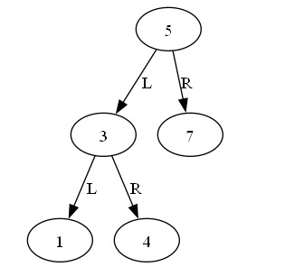
tree.visualize('bst')By executing this you will obtain a PNG file with the image of our graph in the working directory. If we want to view it on IPython, or Jupypter Lab or Notebook, we can use the following code:
from IPython.display import Image, display

display(Image(filename='bst.png'))
You will get the binary tree shown in the figure below.
Main Algorithms – Tree Traversal
Binary tree traversals are fundamental operations that allow you to visit all the nodes of the tree in a certain order. There are three main types of crossings: In-Order, Pre-Order and Post-Order. Each of them defines a different way of visiting nodes, influencing the order in which they are explored.
1. In-Order Traversal:
- In an in-order traversal, you visit the left node, then the current node, and finally the right node.
- Visit order is often used with binary search trees (BSTs) because it ensures that nodes are visited in ascending (or descending) order of value.
   def in_order_traversal(root):
       if root:
           in_order_traversal(root.left_child)
           print(root.value)
           in_order_traversal(root.right_child)
2. Pre-Order Traversal:
- In a pre-order traversal, you first visit the current node, then the left node, and finally the right node.
- Useful for copying tree structure, calculating prefix expressions, or performing preprocessing operations.
   def pre_order_traversal(root):
       if root:
           print(root.value)
           pre_order_traversal(root.left_child)
           pre_order_traversal(root.right_child)
3. Post-Order Traversal:
- In a post-order traversal, the left node is visited first, then the right node, and finally the current node.
- It can be used to perform post-processing operations, such as memory deallocation.
   def post_order_traversal(root):
       if root:
           post_order_traversal(root.left_child)
           post_order_traversal(root.right_child)
           print(root.value)
Example of Use:
# Creating a sample binary tree
tree = BinarySearchTree()
tree.insert(5)
tree.insert(3)
tree.insert(7)
tree.insert(1)
tree.insert(4)

# In-Order crossing
print("In-Order Traversal:")
tree.in_order_traversal()  # Output: [1, 3, 4, 5, 7]

# Pre-Order Crossing
print("\nPre-Order Traversal:")
tree.pre_order_traversal()  # Output: [5, 3, 1, 4, 7]

# Post-Order Traversal
print("\nPost-Order Traversal:")
tree.post_order_traversal()  # Output: [1, 4, 3, 7, 5]
In this example, we show how to perform each of the traversals on a binary search tree. Modify the code to suit your specific needs.
Main Algorithms – Binary Search Tree (BST) Search
Searching a Binary Search Tree (BST) is a fundamental operation that uses the ordered structure of the tree to find a specific element efficiently. Binary search trees are designed such that for each node, all nodes in the left subtree have lower values, while all those in the right subtree have higher values. This feature greatly simplifies the search operation.
Description of the Search Algorithm in a BST:
Start from Root: The search operation starts from the root of the tree.
Compare with Current Node Value: Compare the value to search for with the current node value.
Choice of Route:
- If the searched value is equal to the value of the current node, the element has been found, and the operation ends successfully.
- If the value searched for is less than the value of the current node, continue searching in the left subtree.
- If the value searched for is greater than the value of the current node, continue searching in the right subtree.
Repeat Process: Repeat steps 2 and 3 recursively in the appropriate subtree until the element is found or a leaf (node with no children) is reached.
Element Not Found: If the element was not found at the end of the search, the algorithm will return an indicative value (for example, None in Python) to indicate that the element is not present in the tree.
Python implementation:
def search_in_bst(root, value):
    # Base case: tree is empty or value is in the root
    if root is None or root.value == value:
        return root
    # If the value is less, search in the left subtree
    if value < root.value:
        return search_in_bst(root.left_child, value)
    # If the value is greater, search in the right subtree
    return search_in_bst(root.right_child, value)
Example of Use:
# Creating an example binary search tree
tree = BinarySearchTree()
tree.insert(5)
tree.insert(3)
tree.insert(7)
tree.insert(1)
tree.insert(4)

# Searching for a value in the tree
searched_value = 4
search_result = search_in_bst(tree.root, searched_value)

if search_result:
    print(f"Element {searched_value} found in the tree.")
else:
    print(f"Element {searched_value} not found in the tree.")
In this example, the search algorithm is used to search for the value 4 in the binary search tree. The result is then printed for illustrative purposes.
Main Algorithms – Insertion and Deletion in Binary Trees
Inserting and deleting nodes in a Binary Tree are essential operations that maintain the structure and ordered property of the tree. Inserting a new node is necessary when you want to add an element to the tree, while deleting is useful for removing a specific node from the tree without affecting the binary structure and ordering.
Insertion into a Binary Tree:
The binary tree insertion algorithm involves finding the correct place for the new node within the tree based on its value. After the search, the node is inserted as a child of the found node.
def insert_into_tree(root, value):
    # Base case: tree is empty or leaf node
    if root is None:
        return Node(value)

    # Insert into the left subtree if the value is smaller
    if value < root.value:
        root.left_child = insert_into_tree(root.left_child, value)
    # Insert into the right subtree if the value is greater
    elif value > root.value:
        root.right_child = insert_into_tree(root.right_child, value)

    return root
Deletion from a Binary Tree:
The deletion operation in a binary tree is more complex than the insertion operation and involves several cases to handle. In general, we look for the node to delete and, depending on the number of children of the node, we perform the deletion appropriately.
def delete_from_tree(root, value):
    # Base case: tree is empty
    if root is None:
        return root

    # Search for the node to be deleted in the left subtree
    if value < root.value:
        root.left_child = delete_from_tree(root.left_child, value)
    # Search for the node to be deleted in the right subtree
    elif value > root.value:
        root.right_child = delete_from_tree(root.right_child, value)
    # Node to be deleted found
    else:
        # Case 1: Node with no child or only one child
        if root.left_child is None:
            return root.right_child
        elif root.right_child is None:
            return root.left_child

        # Case 2: Node with two children
        # Find the smallest (or largest) successor (or predecessor) in the right (or left) subtree
        root.value = find_min_value_node(root.right_child).value
        # Delete the successor (predecessor) in the right (left) subtree
        root.right_child = delete_from_tree(root.right_child, root.value)

    return root

def find_min_value_node(node):
    current = node
    while current.left_child is not None:
        current = current.left_child
    return current
Example of Use:
# Creating an example binary search tree
tree = BinarySearchTree()
tree.insert(5)
tree.insert(3)
tree.insert(7)
tree.insert(1)
tree.insert(4)

# Inserting a new node
new_value = 6
tree.root = insert_into_tree(tree.root, new_value)

# Deleting an existing node
node_to_delete = 3
tree.root = delete_from_tree(tree.root, node_to_delete)
In this example, insertion and deletion operations are performed on a binary search tree. Modify the code to suit your specific needs.
Balancing Binary Trees and Introduction to AVL Trees
Binary Search Trees (BSTs) can degenerate into inefficient structures, especially with frequent insertions or deletions. To maintain efficient search time, balanced trees have been developed, including AVL Trees.
Balance concept
In an AVL Tree, the difference in height between the left and right subtrees of each node, called the balance factor, must be between -1, 0, and 1. If a node’s balance factor is greater than 1 or less than -1, the tree is unbalanced and requires rotation operations to restore balance.
Implementing an AVL Tree in Python:
Here is a step-by-step guide on how to implement an AVL Tree in Python:
- Define the AVL Node Structure:
- Each node must have a value, a reference to the left subtree, and a reference to the right subtree. Also add the height of the node.
   class AVLNode:
       def __init__(self, value):
           self.value = value
           self.left_child = None
           self.right_child = None
self.height = 1- Define the AVL Tree:
- The AVL Tree will have a reference to the root.
   class AVLTree:
       def __init__(self):
self.root = None- Implementing Rotations:
- Rotations are the key operations to maintain balance.
- Left rotation (left_rotate) and right rotation (right_rotate) are required.
   def left_rotate(self, z):
       y = z.right_child
       T2 = y.left_child

       y.left_child = z
       z.right_child = T2

       z.height = 1 + max(self._get_height(z.left_child), self._get_height(z.right_child))
       y.height = 1 + max(self._get_height(y.left_child), self._get_height(y.right_child))

       return y

   def right_rotate(self, y):
       x = y.left_child
       T2 = x.right_child

       x.right_child = y
       y.left_child = T2

       y.height = 1 + max(self._get_height(y.left_child), self._get_height(y.right_child))
       x.height = 1 + max(self._get_height(x.left_child), self._get_height(x.right_child))

return x- Implement Insertion:
- Insert a node into the tree following the normal process of inserting a BST.
- After insertion, make sure the shaft is balanced.
   def insert(self, root, value):
       # Esegui l'inserimento come in un BST normale
       if not root:
           return AVLNode(value)
       elif value < root.value:
           root.left_child = self.insert(root.left_child, value)
       else:
           root.right_child = self.insert(root.right_child, value)

       # Aggiorna l'altezza del nodo corrente
       root.height = 1 + max(self._get_height(root.left_child), self._get_height(root.right_child))

       # Bilancia l'albero
return self._balance(root, value)- Balancing the Tree After Insertion:
- Use the balance factors to decide which type of rotation to perform.
   def _balance(self, root, value):
       balance = self._get_balance(root)

       # Case 1: Left subtree left imbalance
       if balance > 1 and value < root.left_child.value:
           return self.right_rotate(root)

       # Case 2: Right subtree unbalanced
       if balance < -1 and value > root.right_child.value:
           return self.left_rotate(root)

       # Case 3: Left imbalance of the right subtree
       if balance > 1 and value > root.left_child.value:
           root.left_child = self.left_rotate(root.left_child)
           return self.right_rotate(root)

       # Case 4: Left subtree right-biased
       if balance < -1 and value < root.right_child.value:
           root.right_child = self.right_rotate(root.right_child)
           return self.left_rotate(root)

return root- Other
- Implement deletion and other features as needed.
Esempio di Utilizzo:
Create an AVLTree object and use insert methods and other operations.
avl_tree = AVLTree()
avl_tree.root = avl_tree.insert(avl_tree.root, 10)
avl_tree.root = avl_tree.insert(avl_tree.root, 20)
avl_tree.root = avl_tree.insert(avl_tree.root, 30)
We rewrite all the code, also inserting the graphic visualization, using graphviz.
from graphviz import Digraph
class AVLNode:
def __init__(self, value):
self.value = value
self.left_child = None
self.right_child = None
self.height = 1
class AVLTree:
def __init__(self):
self.root = None
def visualize(self, filename='avl_tree'):
dot = Digraph(comment='AVL Tree')
self._add_nodes(dot, self.root)
dot.render(filename, format='png', cleanup=True)
dot.view()
def _add_nodes(self, dot, root):
if root:
dot.node(str(root.value) + f' ({root.height})')
if root.left_child:
dot.edge(str(root.value), str(root.left_child.value))
self._add_nodes(dot, root.left_child)
if root.right_child:
dot.edge(str(root.value), str(root.right_child.value))
self._add_nodes(dot, root.right_child)
def _get_height(self, root):
if root is None:
return 0
return root.height
def _get_balance(self, root):
if root is None:
return 0
return self._get_height(root.left_child) - self._get_height(root.right_child)
def left_rotate(self, z):
y = z.right_child
T2 = y.left_child
y.left_child = z
z.right_child = T2
z.height = 1 + max(self._get_height(z.left_child), self._get_height(z.right_child))
y.height = 1 + max(self._get_height(y.left_child), self._get_height(y.right_child))
return y
def right_rotate(self, y):
x = y.left_child
T2 = x.right_child
x.right_child = y
y.left_child = T2
y.height = 1 + max(self._get_height(y.left_child), self._get_height(y.right_child))
x.height = 1 + max(self._get_height(x.left_child), self._get_height(x.right_child))
return x
def insert(self, root, value):
if not root:
return AVLNode(value)
elif value < root.value:
root.left_child = self.insert(root.left_child, value)
else:
root.right_child = self.insert(root.right_child, value)
root.height = 1 + max(self._get_height(root.left_child), self._get_height(root.right_child))
return self._balance(root)
def _balance(self, root):
balance = self._get_balance(root)
if balance > 1:
if root.left_child and value < root.left_child.value:
return self.right_rotate(root)
if root.left_child and value > root.left_child.value:
root.left_child = self.left_rotate(root.left_child)
return self.right_rotate(root)
if balance < -1:
if root.right_child and value > root.right_child.value:
return self.left_rotate(root)
if root.right_child and value < root.right_child.value:
root.right_child = self.right_rotate(root.right_child)
return self.left_rotate(root)
return root
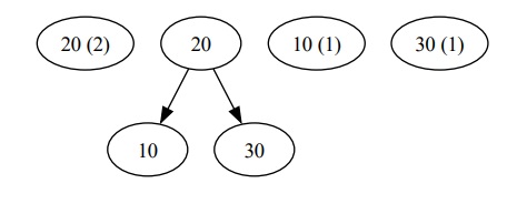
# Example usage:
avl_tree = AVLTree()
avl_tree.root = avl_tree.insert(avl_tree.root, 10)
avl_tree.root = avl_tree.insert(avl_tree.root, 20)
avl_tree.root = avl_tree.insert(avl_tree.root, 30)
avl_tree.visualize('avl_tree_operations')
Running you get the following image:
Remember that this is just a basic guide. Complete management of insertions, deletions, and other aspects may require greater complexity in your code. Additionally, existing libraries in Python, such as avl_tree in the bintrees module, often make it easier to implement AVL trees.