OpenCV & Python – Canny Edge Detection

Introduction

As promised, here is another article in a series of articles about the world of OpenCV and Python development. In a previous article you have already seen the concept of edge detection, this article will show you a particular algorithm called Canny Edge Detection.

If you see more, this is the previous post:

• Edge Detection and Image Gradient Analysis

Canny Edge Detection

In the overview of the algorithms developed for the edge detection, the Canny Edge Detection is quite popular, and owes its name to who developed it, John F. Canny.

This algorithm has a number of interesting features, in fact, is an multistage algorithm:

• Noise Reduction
• Finding Intensity Gradient
• Non-Maximum soppression
• Hysteresis Thresholding

The first stage requires the removal of noise from the image (Noise Reduction), since the edge detection can be influenced by its presence. So to do this, the algorithm uses a 5×5 Gaussian filter for the removal (reduction) of the background noise.

Then the second stage involves the search of the image Intensity Gradient. The image is filtered with a Sobel kernel both in vertical and horizontal direction, thus obtaining the first derivatives in the two directions (Gx and Gy). From these two images, you then find the edge gradient G.

and the gradient direction for each pixel

,

The gradient direction is always perpendicular to the edge. It is rounded to 1 for the four angles that represent the two diagonal directions, and the vertical and horizontal.

The next stage is the Not-maximum Suppression, where some unwanted pixels are removed so they will not be confused as edge. To do this, the entire image is analyzed, checking if each pixel is a local maximum in the direction of the gradient relative to its area.

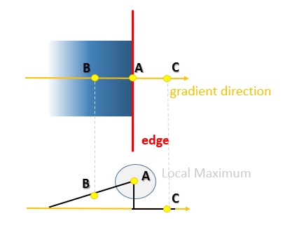
If you look at the figure above, you can see how the analysis is performed. Point A is located on the Edge considered in the vertical direction. You already know that the gradient direction is perpendicular to edge. So the points B and C are analyzed. These points are located on the direction of the gradient. At this point, the point A is compared with the points B and C to see if it forms a local maximum. If it is the local maximum, then it is considered in the next stage, otherwise it is removed, being set to zero.

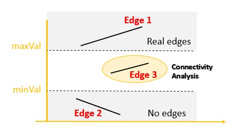
Finally the last stage is the application of the Hysteresis Thresholding. In this final stage the algorithm determines which edges are real edge and and those who are not at all. For this you must determine two threshold values, the minVal the minimum threshold, and maxVal the maximum threshold. Any edge with an intensity gradient greater than maxval is sure to be an edge, and those with a value less than minVal will be discarded, because they are nor real edge. For all other edge that may be found in the range between these two threshold values, are subjected to a further analysis, establishing whether they are real edges through their connectivity. If they are connected to an edge of those already detected, then it is also considered as such, otherwise discarded.

Before you start programming

First to run the code in this article, certain requirements must be met.

Activate the virtual environment in which you have compiled and installed the OpenCV library.

source ~/.profile
workon cv
(cv) $

If you have not yet installed OpenCV, follow the installation procedure described in this article.

In addition, to improve the display of multiple images at once, you will use the matplotlib library. If you have not yet installed on your virtual environment, you can do this by typing

pip --no-cache-dir install matplotlib

Then install the Tkinter package required for the proper functioning of matplotlib.

sudo apt-get install python-tk

You do some testing on a color image, full of edges and color gradients. Download the following file (if you have not already done in the previous examples), and save it as logos.jpg.

Programming the Canny Edge Detection with Python

In OpenCV, this algorithm for the edge detection is already implemented and you can simply use it calling the cv2.Canny() function.

cv2.Canny(image, minVal, maxVal)

This function takes three arguments. The first argument is precisely the image to be analyzed, the second and third arguments are the values of minVal and maxVal respectively, which you have seen earlier.

import cv2
import numpy as np
from matplotlib import pyplot as plt

img = cv2.imread('logos.jpg',0)
edges = cv2.Canny(img,100,110)

plt.subplot(2,1,1),plt.imshow(img,cmap = 'gray')
plt.title('Original Image'), plt.xticks([]), plt.yticks([])
plt.subplot(2,1,2),plt.imshow(edges,cmap = 'gray')
plt.title('Canny Edge Detection'), plt.xticks([]), plt.yticks([])

plt.show()

Running the code you will get the following results.

Other tests on a picture

Now you will perform an edge detection analysis on a picture, rich of details and contours. In this regard I chose the gears of a clock.

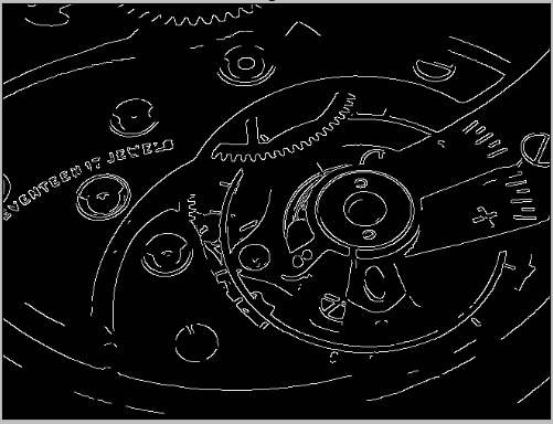
I will use this picture to see the edges selected as varying the minVal and and maxVal threshold values. Here are the results obtained.

These are the edges detected with standard values (minVal = 100, maxVal = 200). As you can see the outlines (edges) of the mechanism have been well identified.

Moving on to a threshold with higher threshold values, you can see that several details are lost, and many outlines become rough. (minVal = 300 and maxVal = 350).

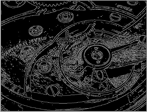
Moving on in the opposite case, using a threshold with too low values, the algorithms detects too many “false” contours as real and the image is enhanced by too many unnecessary details. (minVal = 30 and maxVal = 35).

Conclusions

As you saw in this article, the application of the algorithm Canny Edge Detection is really very simpleprecisely thanks to the OpenCV library. In other articles in this series, you can even go deeper into the topic of edge detection.