Mathematica with raspberry juice – Meccanismo Complesso

Post Views: 2,558

Did you ever consider that Rasperry Pi and Mathematica could work together?

I recently wrote an article on the site electroYou about this topic, and I was asked to propose it to the Meccanismo Complesso community .

I hope that this article will spark interest for all those who are interested in the world of modeling or even for those who are approaching to the world of Raspberry Pi for the first time.

In this article I will explain what hardware you need, how to download this software, how to install and how to use it.

If you are interested, you can download and install the latest release of Mathematica from Wolfram Foundation’s website (it is free), on your Raspberry Pi.

It is a non-limited version, with all 5000 and beyond Mathematica functions working without expire and with special features designed specifically for the Raspberry Pi. It is possible to run Mathematica from your Raspberry Pi in text mode, from a local or remote terminal, in graphical mode, locally or remotely and in kernel-remote mode, even though the latter mode is subject to purchase of a licensed version of Mathematica.

What to buy for use Mathematica on Raspberry Pi

Main components

A Raspberry Model B (with connector Ethernet and 512MB of memory on board), about 35 €.
A micro USB wall adapter that delivers stabilized 5V and 1A at least, few €.
An SD card with at least 16GB of memory (preferably 32GB, working with Mathematica, you will find that the SD card is like the airstrip for pilots of aircraft: it is never too much). The faster the SD card is that you purchase, the faster the Raspberry Pi will be: purchase one with a transfer rate of at least 30MB/s, I assure you that you will not regret, from 10 to 20 €.
A case (also plastic, right to protection) for your new liltte Raspberry!
If you intend to use the GPIO, make sure you buy one that has the slot at the side for the flat cable, otherwise you can obtain it by cutting a slot on one side of the container, from 5 € (plastic) to 50 € (aluminum).

raspberry_mathematica — Fig.1: PiBow Container with slot, but there are many other types

Cables and Connectors

If you use the Raspberry Pi as a terminal, you can connect it to your home router with a simple RJ45 cable. You can also connect it directly to your PC, using cables either Straight type or Crossed type, since modern PCs can understand what type of cable has been used, adapting themself accordingly. Just in case you have a very old PC you have to use a cable of Crossed type. This is the configuration that I have adopted it too, because I use it remotely via SSH (console) or via RDP (Remote Desktop).

If you want to use the Raspberry Pi alone (as a stand-alone computer in practice) in addition to the RJ45 cable you will also have a keyboard and a USB mouse (in this case it might be useful to buy a USB hub, since the Raspberry Pi has only two USB slots and the possibility to have a free USB slot to save data on a memory stick could be very useful), and finally you’ll also need a HDMI cable or a videocomposite signal cable to connect the video output to the TV at home.

During the installation procedure, however, you will have to necessarily use it as a stand-alone computer since remote services are not yet available.

If you want to use the Raspberry Pi to do some experiments on breadboard, it would be better if you buy an Adafruit!, at a cost of two or three euro, basically it is a small PCB (see Fig. 2):

raspberry_mathematica02 — Fig.2: an adafruit!

If you want to work on a stripboard, it is enough to buy a 26-pin IDC connector.

In both cases, you’ll also need a piece of flat cable (see Fig.3) headed at the ends with two IDC connectors for flat with 26-pins, you can make by yourself or buy it already made out for the price of one or two euros.

raspberry_mathematica03 — Fig.3: flat cable with 26-pins and 2 IDC connectors

I would say that the expenditure is made and, in the end, you have not spent too much!

Introduction to Mathematica

Explain what is Mathematica in a few lines, it is really impossible.

Why market leaders are willing to pay almost $10k every 16 kernel of this package (the solution to a modern problem of tensor calculus of nonlinear differential equations with partial derivatives requires many highly parallel computational kernels, to be executed in acceptable time, using very powerful machines), not to mention all the add-ons and optional packages for calculation and the assistance to developers that are sold separately?

Simply because … not buying it they would spend more!

Today, mathematical modeling allows to make predictions very accurately and powerfully, relatively to the physical problem in the subject of study, but requires software products as accurate and powerful, they are also able to perform calculations in symbolic mode. They must also be able to integrate an advanced programming language and interface in languages such as C or C + +. They also need to be able to work in parallel with decomposing the problem into simpler pieces and interact in an intelligent way so that partial results found by a machine should not be recalculated from another machine, all while the calculation is still in progress.

Mathematica is all of this: it is a numerical and symbolic computing environment, it is a powerful interpreted language, both logical and functional and performs pattern recognition: pattern-matching. Virtually all of the libraries of internal functions, then, can be used to create new packages to expand the internal functions of Mathematica.

Imagine what Mathematica has become, then, over the years, since its first release in 1988 until today, with hundreds of programmers around the world who have consistently continued to develop its functions …

And today … we can legally use it free of charge or, at most, the price of a raspberry!

Installing Mathematica on Raspberry Pi

To be able to install Mathematica on your Raspberry Pi, you must first install the operating system Raspbian.

Those who have purchased a pre-formatted SD card along with the Raspberry Pi will find within the Mathematica software installation package NOOB. The package can also be downloaded directly from the website of the Raspberry Foundation. In this case, simply follow the installation instructions after starting the Raspberry with the inserted SD (but remember to make a backup first!).
If you already have the operating system installed, but not yet Mathematica, is absolutely not the case reinstalling all over again, just follow these simple instructions: 1. First, we update the various packages of our Raspberry to the latest release (it would be appropriate to do this every so often) by typing: sudo apt-get update && sudo apt-get upgrade Put in mind that if it is the first time I made this update from when you installed it, it may take a long time before the Raspberry Pi complete the operation. It is possible that the Raspberry Pi asks you to confirm the installation, during the procedure, in which you will answer Y. 2. Once the update is complete, you can move on to installing Mathematica, with the command: sudo apt-get install wolfram-engine At this point you just need to confirm … and wait patiently!

After installation, remember to make the second backup.
By the way, since, if you want to backup, you must turn off the system and remove the SD card, I remind you that the proper way to stop the Raspberry Pi is to type the command:sudo poweroff

Especially if you are a beginner, having a backup will save you much more time if you inadvertently do some kind of trouble!

Mathematica

First look

We now have a complete working version of Mathematica, hooray!
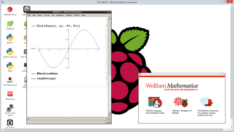
The desktop of the Raspberry Pi is roughly this:

raspberry_mathematica05 — Fig.4: Raspberry’s desktop

The first icon on the top left is Mathematica. Start it!

After you start Mathematica (it will take a few seconds for Mathematica to load all modules) you will see two windows (see Fig. 5).

The first window is called Notebook (on the left) and allows you to enter commands and view the answers provided by the kernel, which is a text-based application that is started secretly and contains the engine of the program. On the right you have another window that is called Helper and is basically a help window. It is still very convenient to have it.

raspberry_mathematica06 — Fig.5: Notebook and Helper on desktop

The first command

If you try to type the command:$MachineName

you will get an answer: raspberrypi.
In practice you have asked Mathematica to tell you about what machine is running the kernel and it said that it is running on the Raspberry Pi. It is not certain that it must always be so.

The first graph

As a second test, you can type the command:Plot[Sin[x],{x,-Pi,Pi}]

You will get a graph of the function sin(x) between -π and π (see the Notebook window in Fig.5).
With the functionTiming[]

you can measure the time Mathematica takes to perform the required calculation.
This feature becomes extremely convenient to do some comparison on the computation time used on a PC and on a Raspberry Pi. By typing:Timing[Plot[Sin[x],{x,-Pi,Pi}]]

it turns out that the computation time on my PC (Intel i7-3520M 2.9GHz, 12GB RAM, Windows 8 64bit) is 0.015s, while on the Raspberry Pi (B type) is 0.53s.
Obviously, the Raspberry Pi is much slower, but it’s still usable.
You can do something more complicated, such as a drawing in 3D, and then you can measure the time necessary to the operation. Type:Timing[Plot3D[Sin[x^2 + y^2], {x, -Pi, Pi}, {y, -Pi, Pi}]]

you obtain:

raspberry_mathematica07 — Fig.6: The ‘eggcup’

The collage shows that my PC takes 0.078s, instead, the Raspberry Pi 3.21s. Not bad, all things considered.

A Bode diagram

You can try to do something even more difficult, for example, a Bode diagram. I choose to plot the two functions, in magnitude and phase:

Insert the following code:

Timing[
    BodePlot[
      {1/(s (s + 10)), ((s + 1))/((s + 100) (s + 10000)) }, 
      plotLabel -> {"Magnitude Plot", "Phase Plot"}, 
      ImageSize -> 550,
      Frame -> True, 
      PlotStyle -> {Directive[Thick, ColorData[20, 1]], Directive[Thick, ColorData[20, 9]]}, 
      Frame -> False, 
      AspectRatio -> 1/2.25, 
      GridLines -> Automatic, 
      GridLinesStyle -> Directive[GrayLevel[0.7],Dashed]
    ]
]

Timing:

Raspberry = 5.14s
PC = 0.094s

A Nyquist diagram

Try to make the Nyquist plot for the first transfer function:

Timing[
     NyquistPlot[1/(s (s + 10)), 
         ImageSize -> 250, 
         Frame -> True, 
         PlotStyle -> {Directive[Thick, ColorData[20, 1]], 
         Directive[Thick, ColorData[20, 9]]}, 
         Frame -> False, 
         GridLines -> Automatic, 
         GridLinesStyle -> Directive[GrayLevel[0.7],Dashed]
        ]
]

Timing:

Raspberry = 5.99s
PC = 0.11s

A Nichols diagram

You can even plot the Nichols diagram:

Timing[
  NicholsPlot[1/(s (s + 10)), 
    ImageSize -> 350, 
    Frame -> True, 
    PlotStyle -> {Directive[Thick, ColorData[20, 1]], 
    Directive[Thick, ColorData[20, 9]]}, 
    Frame -> False, 
    GridLines -> Automatic, 
    GridLinesStyle -> Directive[GrayLevel[0.7], Dashed]
    ]
]

Timing:

Raspberry = 1.84s
PC = 0.031s

Solving linear differential equations with ordinary derivatives

Now try to solve a linear differential equation of the first order, for example, finding the voltage across a capacitor to which a voltage step is applied via a voltage generator.

The code to put in Mathematica is:

Clear[Tau];
Clear[E1];
Timing[
 f = Vc[t] /. 
   Simplify[
     DSolve[{Vc'[t] == (E1 - Vc[t])/Tau, Vc[0] == 0}, Vc[t], t]][[1]];
 E1 = 12;
 Tau = 0.1;
 Plot[f, {t, 0, 1},
  ImageSize -> 550,
  AxesLabel -> {"t", "Vc(t)"},
  PlotStyle -> Directive[Thick, ColorData[20, 1]],
  Frame -> False,
  AspectRatio -> 1/GoldenRatio,
   GridLines -> Automatic,
   PlotRange -> {0, 13},
   GridLinesStyle -> Directive[GrayLevel[0.7], Dashed],
   AxesStyle -> {Directive[Blue, 15], Directive[Blue, 15]}
   ]
  ]
Clear[Tau];
Clear[E1];

Assuming a generator with a voltage of 12V and a time constant equal to 100ms you get this graph:

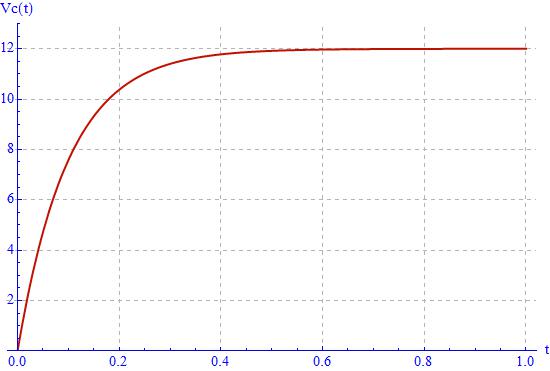
By analyzing the code you can see that I did get the solution to Mathematica symbolically, in fact, printing it, you get:

V_C(t)=E_1\left(1- e^{-\frac{t}{\tau}} \right )

Let us now analyze the computation time:

Raspberry = 2.51s
PC = 0.015s

If the forcing is cosinusoidal for t> 0, it follows that:

Clear[Tau];
Clear[Omega];
Clear[Vmax];
Timing[
 f = Vc[t] /. 
   Simplify[
     DSolve[{Vc'[t] == (Vmax*Cos[Omega*t] - Vc[t])/Tau, Vc[0] == 0}, 
      Vc[t], t]][[1]];
 Vmax = 230;
 Tau = 0.001;
 Omega = 314;
 Plot[{f, Vmax*Cos[Omega*t]}, {t, 0, 0.04},
  ImageSize -> 550,
  AxesLabel -> {"t", "Vc(t)"},
  PlotStyle -> {Directive[Thick, ColorData[20, 1]], 
    Directive[Dotted, ColorData[1, 2]]},
  Frame -> False,
  AspectRatio -> 1/GoldenRatio,
   GridLines -> Automatic,
   GridLinesStyle -> Directive[GrayLevel[0.7], Dashed],
   AxesStyle -> {Directive[Blue, 15], Directive[Blue, 15]}
   ]
  ]
Clear[Tau];
Clear[Omega];
Clear[Vmax];

placing:

Vmax = 230 V;
Tau = 0.001 s;
Omega = 314 rad/s;

you obtain:

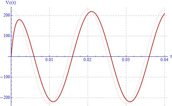
It may be noted that the dotted line corresponds to the voltage applied to the circuit by the generator. Let us now analyze the computation time:

Raspberry = 3.78s
PC = 0.093s

The solution found by Mathematica is:

V_C(t)=\text{Vmax}\frac{\omega \tau \sin (\omega t)+\cos (\omega t)-e^{-\frac{t}{\tau}}}{\omega^2 \tau^2+1}

Parameterizations, animations and LDPE

Suppose, for example, to have solved the wave equation and want to understand a little about how things are from the physical point of view.
The Manipulate command allows you to play with the parameters of an equation by providing the sliders. Sometimes I use it, especially when I have to figure out what the equation that I have just solved, means …
Try to enter this code:

Manipulate[
 Show[
  Plot[
   Cos[1*t - x/\[Lambda]], {x, -5, 0},
   PlotRange -> {{-5, 5}, {-2, 2}},
   PlotStyle -> Black],
  Plot[\[CapitalGamma]*Cos[1*t + x/\[Lambda]], {x, -5, 0},
   PlotRange -> {{-5, 5}, {-2, 2}},
   PlotStyle -> Red],
  Plot[(1 - \[CapitalGamma]) Cos[1*t - x/\[Lambda]], {x, 0, 5},
   PlotRange -> {{-5, 5}, {-2, 2}},
   PlotStyle -> Blue],
  ImageSize -> {400, 300}],

 {{\[Lambda], 1, "wavelength \[Lambda]"}, .1, 5, ImageSize -> Tiny},
 {{\[CapitalGamma], .1, "reflection coefficient \[CapitalGamma]"}, 0, 
  1, ImageSize -> Tiny},
 {{t, 0, "time"}, 0, Infinity, ControlType -> Trigger},
 AutorunSequencing -> {2, 3, 4}]

You will get a window like this:

raspberry_mathematica15 — Fig.7: the Manipulate command generates cursors

As you can see in Figure 7, at x = 0 there is a discontinuity, the wave drawn in black is the incident wave, the reflected wave is in red, while the blue one has the transmitted wave.
By varying the available sliders you can see what happens by changing the wavelength and the reflection coefficient. Pressing the button (play) you will get an animation preset parameters.
To get an idea of what you can get, here is an animation done by placing the reflection coefficient equal to 0.5:

raspberry_mathematica_16 — Fig.8: Graphic solution of the monodimensional equation of the waves with reflection coefficient of 0.5

Timing:

Raspberry Pi = 0.02s
PC < eps (practically it gives me zero)

Matrices

One problem that I solved was the inversion of a matrix of the type:

Unfortunately Mathematica can not yet reverse this matrix varying its size by finding a general formula for doing so, however, it could be of great help to verify the goodness of the solution found.
Setting the function containing the solution:

f[n_, i_, j_] := 1/3*(1/2^(Abs[i - j]) - 1/(2^(2*n + 2 - i - j)))
M[k_] := Table[f[k, i, j], {i, 1, k}, {j, 1, k}]

You can enjoy yourself to build an inverse matrix of order n by writing M[n]. For example:

Let’s see if reversing the inverse matrix you can obtain again the main matrix. Among other things, you can do so by making a small graphic on the computation time.

I would say that it works. At this point you can use the matrix to make a small program to measure execution times and make a chart. First, let’s see how to create the various points. I gave the command:

vaio = Table[{n, Timing[Inverse[M[n]];][[1]]}, {n, 1, 50}]

on my PC and the command:

raspi = Table[{n, Timing[Inverse[M[n]];][[1]]}, {n, 1, 50}]

on Raspberry Pi, which is the same command given on my PC, with the difference that the resulting vector was called ‘raspi’…

If you have studied all the various commands that I have used, you will notice that vaio and raspi are two matrices containing in the first column the size of the matrix to be inverted and, in the second column, the time taken to reverse it. In practice you have the array of points (x, y), which are useful to make the chart I was looking for.
To do this we use the command ListLinePlot:

ListLinePlot[
 {vaio, raspi},
 ImageSize -> 550,
 AxesLabel -> {"n", "t (s)"},
 PlotStyle -> {Directive[Thick, ColorData[55, 1]], 
   Directive[Thick, ColorData[20, 1]]},
 Frame -> False,
 AspectRatio -> 1/GoldenRatio,
  GridLines -> Automatic,
  GridLinesStyle -> Directive[GrayLevel[0.7], Dashed],
  AxesStyle -> {Directive[Blue, 15], Directive[Blue, 15]},
 PlotLegends -> {"PC", "Raspberry Pi"}
 ]

The result of which is:

mathematica-raspberry-curve — Fig.9: Vaio vs Raspi

Clearly, the PC wins, (in fact, with the PC you need a license for a fee of Mathematica, Stephen Wolfram makes some nice gifts but he is not stupid) but better looking the chart you can see that in about 2.2s you can invert a matrix 40×40, and if you’re willing to wait six seconds, you can reverse a 50×50. After all it is not so bad.

Clearly if you have to invert a 200×200 matrix, you would certainly need to use a PC (which would take us 14.62s. The Raspberry, estimating from the graph, would take more than 13 minutes to calculate).
Note that the time on the graph grows, in both cases, as the cube of n, which is the order of magnitude of time required for the algorithm to invert matrices.

Mathematica commands for Raspberry PI

Superuser mode

Stephen Wolfram wanted to pay homage to fans of Raspberry with specific functions, which allow you to access the hardware system of the Raspberry Pi.
is necessary, however, to be able to access these functions, launching Mathematica in administrator mode, since it will have access to the hardware resources. So, you have to create a desktop icon to launch the Raspberry Mathematica in administrator mode:

Click with the left mouse button over the icon of Mathematica (once);
Type CTRL+C and then CTRL+V;

you will see a window like this:

raspberry_mathematica17 — Fig.10: Just in front of the raspberry, it should appear?

Change the string from Wolfram-Mathematica.desktop to Wolfram-Mathematica-sudo.desktop and click on Rename, who in the meantime has become selectable;

Then click with the right button on the icon created and, from the menu that appears, click on Leafpad (it should be the second item above);
This will open a text editor with the following content:

[Desktop Entry]
Version=1.0
Type=Application
Name=Mathematica
Comment=Technical Computing System
TryExec=mathematica
Exec=/opt/Wolfram/WolframEngine/10.0/Executables/mathematica %F
Icon=wolfram-mathematica
MimeType=application/mathematica;application/vnd.wolfram.cdf;application/mathematicaplayer
Categories=Application;Education;

Change the fourth line with: Name=MathemSudo

and the seventh with: Exec=sudo /opt/Wolfram/WolframEngine/10.0/Executables/mathematica %F

Save and exit.
Now you have an icon to launch Mathematica in administrator mode.

A simple circuit

The first thing we try to do is to drive the LEDs. We are going to connect these LEDs on GPIO port of Raspberry. Try to find this expansion connector:

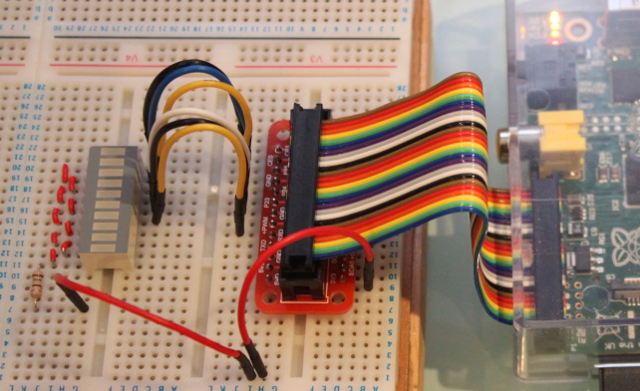
Thus, connect the piece of flat cable (that you procured earlier) to the GPIO. The other end of the connector will be connected to the coupon Adafruit! (previously purchased). You should get a result of this type:

raspberry_mathematica19 — Fig.12: Don’t you see all the mess that I have on my desk, right?

The result seems to be a clean and tidy work, without loose wires that could become detached giving rise to some short circuit.

In this regard, you should be careful to work with the GPIO pins, since the processor A11 on the Raspberry Pi is not made to handle I/O so heavy as it is, for example, implemented on a PIC or on an AVR. An A11 is, in fact, a microprocessor and not a microcontroller.
So, be very careful, if you connect one pin to ground configuring it as an output and then you write a logic one on it, you simply ruine the Raspberry. Same thing if you write a logic zero on a pin linked to V_dd.

In addition, the microprocessor works at 3.3V and none of the I/O is 5V tolerant, so, as before, if you configure an I/O as input and then connect it to 5V, you simply ruin your Raspberry Pi. Each output can provide not more than 16mA, and all together not more than 40mA. For this reason you will light only one LED (red) at a time with a resistor common to all the LEDs equal to 180Ω.
Thus, let’s out our attention to the circuit itself. You have to follow this scheme:

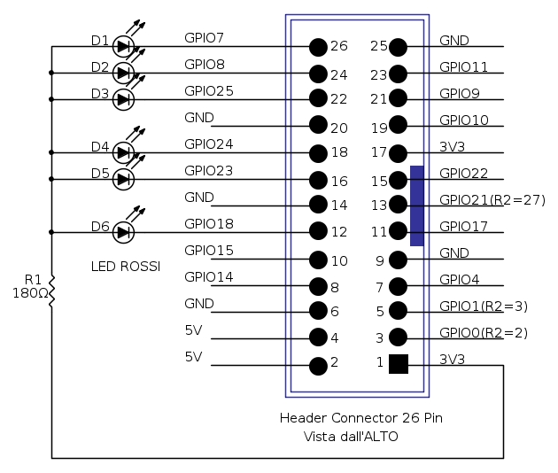
mathematica-raspberry-header — Fig.13: Header Conenctor made with FidoCadJ

In Fig.14 instead I show you how I carried out the installation. I tried to be more tidy as possible:

Fig.12: circuito montato con 6 LED — Fig.14: the circuit with 6 LEDs

The key function available on Mathematica, to write on a pin of Raspberry PI, is:DeviceWrite["GPIO", numero_del_pin -> 1_o_0]

First you need to arrange the pins in a sorted array:pins = {7, 8, 25, 24, 23, 18};

Then it will be sufficient to take the i-th element of the vector to turn on the corresponding LED. Quite simply, you can use the good old command Manipulate already met earlier.
The code becomes:

pins = {7, 8, 25, 24, 23, 18};
Do[DeviceWrite["GPIO", pins[[i]] -> 1], {i, Length[pins]}];
previous = 1;
LEDs[i_] := {
   DeviceWrite["GPIO", pins[[previous]] -> 1];
   DeviceWrite["GPIO", pins[[i]] -> 0];
   previous = i;
   };
Manipulate[LEDs[i], {i, 1, Length[pins], 1}]

The second line, which is the command Do[], is used to turn off all the LEDs (as it is connected, putting the output to 1, the LED turns off). The third line sets the variable previous to 1 and is used to make sure that, once you start the cycle, the LED is lit before it can be turned off.

The fourth line contains the function LEDs, which turns off the previous LED, turns on the required LED and stores the LED on in the previous variable so you can turn off it at the next call.The Manipulate command finally allows us to set the cycle as we want.

Running the code will see this window:

mathematica-raspberry-finestra1 — Fig.15: The manipulate window

If you move the cursor you will see the corresponding LED turning on. If you click on the + indicated by the arrow:

mathematica-raspberry-finestra2 — Fig.16: Click on me!

You will see a small menu but very useful appears:

mathematica-raspberry-finestra3 — Fig.17: menu with extra functions

Let’s explain it from left to right:

In the text area you can write a number, from 1 to 6, corresponding to the number of LED to turn on;
Clicking on – you decrease the number written in the text by one unit ;
The symbol , Play, animates the LED by moving the rod automatically;
Clicking on + you increase the number written in the text by one unit;
Clicking on the double arrows upward you will increase the scanning speed of the LEDs;
Clicking on the double arrows downward you decrease the scanning speed of the LEDs;
The ultimate symbol allows you to switch between the forward scan, backward scan and bidirectional scanning.

Reading the state of a pin

To read the state of a pin you can use the function:DeviceRead["GPIO", pin_da_leggere]

Assemble the following circuit (or add the missing part of the previous one):

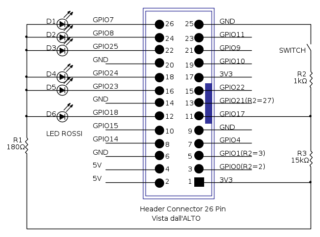
mathematica-raspberry-fidocadj — Fig.18: Header connector 26 Pin

I also inserted a resistance in series to the button / switch to avoid, in case of mistaken to set the GPIO of the Raspberry Pi configuring it as output, rather than as an input, to ruin the port.

In case you want to use a pin as an output, you can write the value to be set directly on the port to be set. It is not so, however, in case you want to read the status of a bit. This is because, by default, the GPIO pins are set as outputs.
It is necessary, in this case, to configure the bits as input, with the statement:DeviceConfigure["GPIO", bit_da_impostare -> "Input"]

If we had a vector you would need to scan it with a Do statement. For example, this program configures the LED bits as inputs, reads them and fills a vector with the scanning of the reading:

sw = 1; i = 1;
pins = {7, 8, 25, 24, 23, 18};
inputs = ConstantArray[-1, Length[pins]];
Do[
 DeviceConfigure["GPIO", pins[[i]] -> "Input"];
 inputs[[i]] = pins[[i]] /. DeviceRead["GPIO", pins[[i]]];
 , {i, Length[pins]}]
inputs

This program instead reconfigures all the bits of the LEDs as outputs, and places them at 1:

pins = {7, 8, 25, 24, 23, 18};
Do[
 DeviceConfigure["GPIO", pins[[i]] -> "Output"];
 DeviceWrite["GPIO", pins[[i]] -> 1];
 , {i, Length[pins]}]

Let us now make a little program that makes the LEDs turning on in sequence until you press the button:

sw = 1; i = 1;
pins = {7, 8, 25, 24, 23, 18};
DeviceConfigure["GPIO", 17 -> "Input"]
While[sw == 1,
 sw = 17 /. DeviceRead["GPIO", 17];
 DeviceWrite["GPIO", pins[[i]] -> 1];
 If[i < Length[pins], i++, i = 1];  DeviceWrite["GPIO", pins[[i]] -> 0];
 Pause[0.2];
 ]
DeviceWrite["GPIO", pins[[i]] -> 1];

It is not the best way to do it, but it is certainly the easiest.

Importing images from the camera to Raspberry Pi

The Raspberry Pi has a connector specially designed to accommodate a small camera.
There are two models, one with 5Mpixel 1080p:

mathematica-raspberry-connettore1 — Fig.19: Camera with 5Mpixel 1080p

and one for night vision, always 5Mpixel 1080p:

mathematica-raspberry-connettore2 — Fig.20: IR Camera with 5Mpixel 1080p

Here is a picture with the camera in its Raspberry connector:

mathematica-raspberry-connettore3 — Fig.21: Raspi and Camera just married

Mathematica allows you to capture an image from the camera with the command:image1 = DeviceRead["RaspiCam"];

At this point in the variable image1 you have the picture and you can manipulate it using a any command of Mathematica.

Serial communications RS232

Mathematica for Raspberry Pi can communicate with the serial port on the GPIO connector (pin 8 and pin 10 TX, RX).
CAUTION: Do not connect a serial directly to any of these pins, which work at 3.3V, without moving the layers or you will ruin the Raspberry Pi.
The first thing you need to do is to open the port of communication. We can use the command:serial = DeviceOpen["Serial",{"/dev/ttyUSB0","BaudRate"->9600}]

You can replace 9600 with the required BaudRate (from 476 Baud up to 31.25MBaud). 115200 is the default BaudRate.
At this point it is possible to read a string of data from the serial port:data = DeviceReadBuffer[serial,"String"]

The command will read from the open serial and fill it with the given string buffer. Or, if you prefer, you can write a string to the serial port:DeviceWriteBuffer[serial,data]

The command will write to the serial port in serial the data string.

Mathematica in remote-kernel mode

If you followed the examples I’ve shown here, trying them directly on Mathematica on your Raspberry Pi, you may have noticed that if you connect to the RDP in Raspberry (with, for example, Windows Remote Desktop) the speed of dialogue with the desktop not is exciting, but things improve a lot if you have the Raspberry Pi connected to the home TV and you are using it with your keyboard and your mouse.
Mathematica allows you, if you have a version on a PC, to use the front-end (GUI only) on your PC, but the kernel of the Raspberry, connecting remotely.
Let’s see how to get access to this tool.
First open Mathematica on your PC, go on Evaluation and then on Kernel Configuration Options.
It will open this little window:

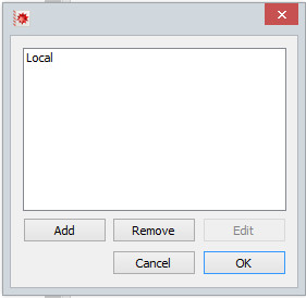
mathematica-raspberry-finestra4 — Fig.22 little windows for great kernels

Click on Add.
At this point you will have to fill out the form that appears by copying the image that I have provided below, with the only exception for Machine Name that will be filled with the IP address of your Raspberry Pi.

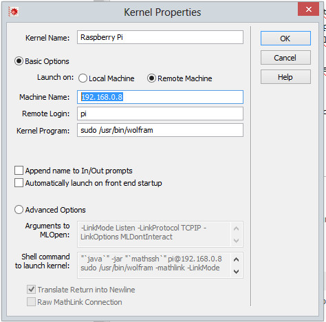
mathematica-raspberry-finestra5 — Fig.23: Fill me!

Click OK. At this point you will return to the previous window, to which the new entry Raspberry Pi is added. Click OK and you will return to Mathematica.
At this point you just have to decide which kernel to use, the local machine kernel or the Raspberry Pi kernel. To decide which kernel to use, go on Evaluation and then on Default Kernel and choose the new entry Raspberry Pi. A window will appear asking for the password to access the Raspberry Pi (by the way … you’ve changed it, right?) And you’re done!
If you give the command: $MachineName

you will get an answer: raspberrypi.

mathematica-raspberry-finestra6 — Fig.24: let’s use the Raspberry kernel!

At this point, if you run on your PC any one of the small programs shown above, for example using the LEDs, you will see the LEDs light on Raspberry.

Mathematica in text mode

Those who use Mathematica professionally, in general, do not often use the GUI, if not to graphically display the results or do the manipulations on data already calculated.
This is because the kernel, alone, is infinitely faster and allows, graphics aside, any calculation and any processing possible with Mathematica.
Personally I found the connection to the Raspberry Pi with Putty SSH (running in text mode) much more profitable than any other solution. It is very fast and allows egregious elaborations.
Once the SSH connection with the Raspberry Pi is established, it is possible to run the Mathematica kernel by simply typing:sudo wolfram

mathematica-raspberry-putty1 — Fig.25: Putty on Raspi

At this point it is possible, GUI part, to use all commands of Mathematica (they are more than 5k). Let’s do some simple calculation using the kernel itself:

mathematica-raspberry-putty2 — Fig.26: Who would have thought it….DirtyDeeds…

If you want to automatically execute a program you can create a text file that contains it and then save it with the extension .m. Suppose you have created the text file LED.m and you want to run it.

From the command line you can type:sudo wolfram -script LED.m

While, if you have already started the kernel, you can just give the command:<< _percorso_\LED.m

When you want to quit, you can exit with the command:Quit (Q uppercase)

Conclusions

In this article I have tried to carry out an overview on how to use Mathematica, and with the excuse of the Raspberry, I introduced a number of specialized functions, both for using them in dedicated minicomputer and for general use.
I dedicate it to all those who wish to approach this program and, more generally, to the world of modeling.
May each day be a beautiful discovery of the physical reality that surrounds you.
I hope you never stop to amaze you.

Installing Mathematica on Raspberry Pi

Mathematica

First look

The first command

The first graph

A Bode diagram

A Nyquist diagram

A Nichols diagram

Solving linear differential equations with ordinary derivatives

Parameterizations, animations and LDPE

Matrices

Mathematica commands for Raspberry PI

Superuser mode

A simple circuit

Reading the state of a pin

Importing images from the camera to Raspberry Pi

Mathematica in text mode

Conclusions

Leave a Reply Cancel reply