The CART algorithm in Machine Learning with Python

Post Views: 58

The CART algorithm

The CART (Classification and Regression Trees) algorithm is a widely used algorithm for building decision trees in machine learning. Decision trees are a form of predictive model that can be used for both classification and regression problems. Here’s how the CART algorithm works and how to use it in Python.

Operation of the CART Algorithm

The goal of the CART algorithm is to recursively divide the training dataset into homogeneous subsets in order to maximize the purity of the classes or minimize the error in predicting the target variable, depending on whether it is a classification or regression problem.

Here is an overview of the main steps of the CART algorithm

Choice of the predictor variable and the division threshold: The CART algorithm begins by selecting the predictor variable (characteristic) and threshold value that maximize the purity of the classes or minimize the error in predicting the target variable. For continuous variables, for example, the threshold might be a value such as 3.5, while for categorical variables, all categories might be tested.
Division of the dataset: Once the variable and the threshold have been chosen, the dataset is divided into two subsets: one containing the examples that satisfy the division criterion and the other containing those that do not.
Calculation of purity or error: A purity or error measure is calculated for each of the two subsets. For example, for classification problems, the Gini index or entropy could be used to measure purity. For regression problems, the mean square error (MSE) could be used).
Recursive repetition: The steps above are repeated recursively for each subset until a stopping criterion is met, for example, when the maximum number of splits has been reached or when all examples belong to the same class (for classification problems) or when the target variation is below a certain threshold (due to regression problems).
Mast Construction: At the end of the recursive process, a complete decision tree is constructed, where internal nodes represent splits based on the predictor variables and leaf nodes represent predictions.

A bit of history

The CART (Classification and Regression Trees) algorithm was developed by Leo Breiman, Jerome Friedman, Richard Olshen, and Charles Stone and was introduced in the 1980s. The main goal of CART is to build binary decision trees that can be used for classification and regression.

The history of CART is linked to the growing need to develop machine learning models that could tackle complex classification and regression problems. The decision tree approach has proven attractive due to its conceptual simplicity and ease of interpretation of results. CART represented a significant step in the evolution of machine learning and paved the way for many variations and improvements in decision tree algorithms.

One of the key aspects of CART is its flexibility in addressing a variety of problems, including those with continuous and categorical variables. Furthermore, the use of impurity criteria such as the Gini index or entropy allowed the selection of predictor variables and cutpoints to be effectively managed.

In addition to being a stand-alone model, the CART approach has also influenced the development of ensemble algorithms such as Random Forest, which relies on combining different decision trees to improve predictive performance.

In the years since, the use of decision trees and their variants has spread to many applications, including data analysis, pattern recognition, text classification, and much more. CART has proven to be a valuable asset in the arsenal of machine learning techniques and remains an important foundation for the development of more complex algorithms in the field of machine learning

The CART algorithm with the scikit-learn library

In Python, you can use the scikit-learn library to implement the CHAID algorithm in the following approaches:

Classification
Regression

CART for Classification problems

The classification problem we face is based on the Iris dataset, where the goal is to classify flowers into one of three species (setosa, versicolor or virginica). Let’s divide the code into steps with descriptions for better understanding:

Step 1: Import libraries and upload dataset:

We start by importing the necessary libraries, loading the Iris dataset, and dividing the data into training and test sets.

import numpy as np
import matplotlib.pyplot as plt
from sklearn.datasets import load_iris
from sklearn.tree import DecisionTreeClassifier
from sklearn.model_selection import train_test_split
from sklearn.metrics import accuracy_score, confusion_matrix, plot_confusion_matrix

# Load the Iris dataset
iris = load_iris()
X = iris.data
y = iris.target

# Divide the dataset into training and test sets
X_train, X_test, y_train, y_test = train_test_split(X, y, test_size=0.2, random_state=42)

Step 2: Create and train a CART model:

Now let’s create a CART model using scikit-learn’s DecisionTreeClassifier and train it on the training data.

# Create a CART template
tree_classifier = DecisionTreeClassifier(random_state=42)

# Train the model on the training data
tree_classifier.fit(X_train, y_train)

Step 3: Make predictions and evaluate the model:

We can now use the trained model to make predictions on the test data and evaluate the model’s performance.

# Make predictions on test data
y_pred = tree_classifier.predict(X_test)

# Calculate the accuracy of the model
accuracy = accuracy_score(y_test, y_pred)
print("Accuratezza del modello:", accuracy)

# View the confusion matrix
confusion_matrix(y_test, y_pred)
plot_confusion_matrix(tree_classifier, X_test, y_test, display_labels=iris.target_names)
plt.title("Matrice di Confusione")
plt.show()

In this example, we built a CART model, made predictions on the test data, and calculated the model’s accuracy. We also visualized the confusion matrix for a more detailed assessment of the model’s performance.

Make sure you have scikit-learn, numpy and matplotlib installed before running the code.

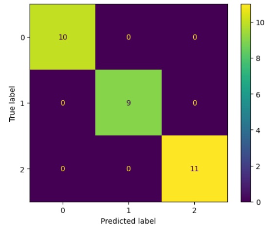
CART for Regression problems

In this example, we will use the Boston Housing dataset to predict the price of homes based on several characteristics. We divide the code into steps with descriptions for better understanding:

Step 1: Import the libraries and load the dataset:

We start by importing the necessary libraries, loading the Boston Housing dataset, and splitting the data into training and test sets.

import numpy as np
import matplotlib.pyplot as plt
from sklearn.datasets import load_boston
from sklearn.tree import DecisionTreeRegressor
from sklearn.model_selection import train_test_split
from sklearn.metrics import mean_squared_error, r2_score

#Load the Boston Housing dataset
boston = load_boston()
X = boston.data
y = boston.target

# Divide the dataset into training and test sets
X_train, X_test, y_train, y_test = train_test_split(X, y, test_size=0.2, random_state=42)

Step 2: Create and train a CART model for regression:

Now let’s create a CART model for regression using scikit-learn’s DecisionTreeRegressor and train it on the training data.

#Create a CART model for regression
tree_regressor = DecisionTreeRegressor(random_state=42)

# Train the model on the training data
tree_regressor.fit(X_train, y_train)

Step 3: Make predictions and evaluate the model:

We can now use the trained model to make predictions on the test data and evaluate the model’s performance using regression metrics such as mean square error (MSE) and coefficient of determination (R^2).

#Make predictions on test data
y_pred = tree_regressor.predict(X_test)

# Calculate the mean square error (MSE)
mse = mean_squared_error(y_test, y_pred)
print("Errore Quadratico Medio (MSE):", mse)

# Calculate the coefficient of determination (R^2)
r2 = r2_score(y_test, y_pred)
print("Coefficient of Determination (R^2):", r2)

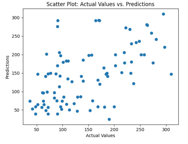
# Displays a scatterplot between actual and predicted values
plt.scatter(y_test, y_pred)
plt.xlabel("Valori Effettivi")
plt.ylabel("Previsioni")
plt.title("Grafico di Dispersione: Valori Effettivi vs. Previsioni")
plt.show()

In this example, we created a CART model for the regression, made predictions on the test data, and evaluated the model using the mean square error (MSE) and the coefficient of determination (R^2). Additionally, we displayed a scatterplot to visually examine predictions versus actual values.