The Fibonacci Series: three different algorithms compared

The efficiency of algorithms plays a central role in software development, directly influencing the performance and responsiveness of applications. In this context, the Fibonacci series provides fertile ground for exploring and comparing different implementation strategies, from the classic recursive approach to more optimized solutions such as iteration and dynamic programming.

[wpda_org_chart tree_id=44 theme_id=50]

This article aims to analyze three main approaches to generate the Fibonacci series in Python: the recursive implementation, the iterative approach and the one based on dynamic programming. Through the comparison of asymptotic complexities and practical performance analysis, we will try to highlight the distinctive characteristics of each method and provide guidance on choosing the most suitable algorithm for specific scenarios.

The decision-making process in adopting an algorithm is crucial to guarantee optimization of resources and an efficient response to the requirements of the problem. We therefore invite the active discovery of optimized solutions, underlining the importance of experimentation and understanding the application context to make informed decisions in the design and implementation of algorithms.

The Fibonacci series

The Fibonacci series is a sequence of integers in which each number is the sum of the previous two, starting with 0 and 1. The sequence is defined as follows:

The sequence begins with 0, 1, 1, 2, 3, 5, 8, 13, 21, and so on. Each subsequent number is the sum of the two previous numbers. The sequence was introduced to Europe by Leonardo Fibonacci in his book “Liber Abaci” in 1202, but the sequence was already known in India much earlier.

The Fibonacci series exhibits several interesting mathematical properties. Some of them include:

• Recurrence Properties:
  
• Asymptotic Limit:
  As (n) increases, the ratio between and converges to the golden ratio

Where is the golden ratio, approximated to approximately 1.6180339887.

The Fibonacci series has a notable presence in both mathematics and computer science. In mathematics, the sequence manifests itself in numerous natural phenomena, such as the arrangement of leaves on a branch, the petals of flowers and the spiral of some shells. Furthermore, the Fibonacci series is related to the concept of the golden ratio, with the ratio between successive numbers converging to the approximate value of 1.6180339887.

In computer science, the Fibonacci series is often used as an example to illustrate fundamental concepts such as recursion, dynamic programming, and algorithmic complexity. Algorithms for generating the Fibonacci series provide fertile ground for exploring different problem-solving and optimization strategies.

Its ubiquitous presence in nature and its relevance in computing make the Fibonacci series a fascinating and crucial topic that connects the world of pure mathematics with practical applications in science and technology.

The Three Proposed Algorithms

that is, we implement several algorithms to generate the Fibonacci series in Python and compare them based on asymptotic notations. The main approaches are:

• recursive
• iterative
• with dynamic programming.

Let’s see some example code of the three different algorithms, reported in the form of 3 different functions.

Recursion:

def fibonacci_recursion(n):
    if n <= 1:
        return n
    else:
        return fibonacci_recursion(n-1) + fibonacci_recursion(n-2)

Iterative

def fibonacci_iterative(n):
    a, b = 0, 1
    for _ in range(n):
        a, b = b, a + b
    return a

Programmazione dinamica:

def fibonacci_dynamic(n):
    fib = [0] * (n + 1)
    fib[1] = 1
    for i in range(2, n + 1):
        fib[i] = fib[i - 1] + fib[i - 2]
    return fib[n]

We can now compare the performance of these algorithms using running time and looking at asymptotic notations.

import time

def measure_time(func, *args):
    start_time = time.time()
    result = func(*args)
    end_time = time.time()
    execution_time = end_time - start_time
    return result, execution_time

n = 30 
result_recursion, time_recursion = measure_time(fibonacci_recursion, n)
result_iterative, time_iterative = measure_time(fibonacci_iterative, n)
result_dynamic, time_dynamic = measure_time(fibonacci_dynamic, n)

print(f"Recursion: {time_recursion} sec, Result: {result_recursion}")
print(f"Iterative: {time_iterative} sec, Result: {result_iterative}")
print(f"Dynamic: {time_dynamic} sec, Result: {result_dynamic}")

Executing you will get the following result:

Recursion: 0.28981590270996094 sec, Result: 832040
Iterative: 0.0 sec, Result: 832040
Dynamic: 0.0 sec, Result: 832040

Let’s look at it better from a graphical point of view. Rewriting the code in the following form:

import time
import matplotlib.pyplot as plt

def fibonacci_recursion(n):
    if n <= 1:
        return n
    else:
        return fibonacci_recursion(n-1) + fibonacci_recursion(n-2)

def fibonacci_iterative(n):
    a, b = 0, 1
    for _ in range(n):
        a, b = b, a + b
    return a

def fibonacci_dynamic(n):
    fib = [0] * (n + 1)
    fib[1] = 1
    for i in range(2, n + 1):
        fib[i] = fib[i - 1] + fib[i - 2]
    return fib[n]

def measure_time(func, *args):
    start_time = time.time()
    result = func(*args)
    end_time = time.time()
    execution_time = end_time - start_time
    return result, execution_time

def plot_fibonacci_time_complexities(max_n):
    n_values = list(range(2, max_n + 1))
    times_recursion = []
    times_iterative = []
    times_dynamic = []

    for n in n_values:
        _, time_recursion = measure_time(fibonacci_recursion, n)
        _, time_iterative = measure_time(fibonacci_iterative, n)
        _, time_dynamic = measure_time(fibonacci_dynamic, n)

        times_recursion.append(time_recursion)
        times_iterative.append(time_iterative)
        times_dynamic.append(time_dynamic)

    plt.plot(n_values, times_recursion, label='Recursive')
    plt.plot(n_values, times_iterative, label='Iterative')
    plt.plot(n_values, times_dynamic, label='Dynamic')

    plt.xlabel('n (Fibonacci value)')
    plt.ylabel('Execution time (secs)')
    plt.title('Trend of the algorithms for the Fibonacci series')
    plt.legend()
    plt.show()

#Specify the maximum value of n for the graph
max_n = 30
plot_fibonacci_time_complexities(max_n)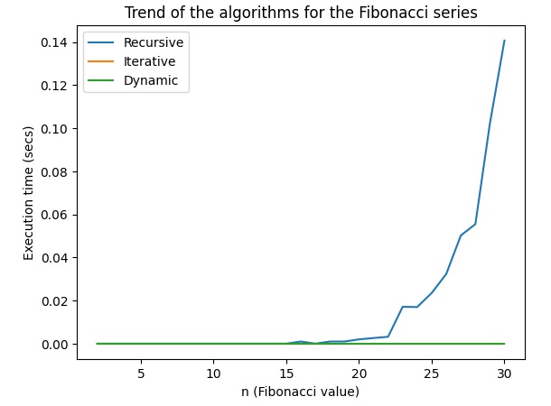

It is important to note that the recursive approach quickly becomes inefficient for larger values of n due to its exponential complexity. Dynamic programming is generally more time efficient than the iterative or recursive approach, especially for large inputs, due to its linear complexity.

Practical comparison between iteration and dynamic programming

In the previous example we saw how the recursion algorithm quickly becomes inefficient. But as regards the other two algorithms it is difficult to make evaluations, given that the execution times are equal to 0 (too fast) and the trends are completely flat. The difference between the iterative and dynamic programming approaches may be more evident for larger values of n. Furthermore, we could use the timeit library to obtain more accurate measures of execution time. Here is an updated version of the code:

import timeit
import matplotlib.pyplot as plt

def fibonacci_iterative(n):
    a, b = 0, 1
    for _ in range(n):
        a, b = b, a + b
    return a

def fibonacci_dynamic(n):
    fib = [0] * (n + 1)
    fib[1] = 1
    for i in range(2, n + 1):
        fib[i] = fib[i - 1] + fib[i - 2]
    return fib[n]

def measure_time(func, *args):
    return timeit.timeit(lambda: func(*args), number=1000)

def plot_fibonacci_time_complexities(max_n):
    n_values = list(range(2, max_n + 1))
    times_iterative = []
    times_dynamic = []

    for n in n_values:
        time_iterative = measure_time(fibonacci_iterative, n)
        time_dynamic = measure_time(fibonacci_dynamic, n)

        times_iterative.append(time_iterative)
        times_dynamic.append(time_dynamic)

    plt.plot(n_values, times_iterative, label='Iterative')
    plt.plot(n_values, times_dynamic, label='Dynamic')

    plt.xlabel('n (Fibonacci value)')
    plt.ylabel('Tempo di esecuzione (secondi)')
    plt.title('Practical comparison')
    plt.legend()
    plt.show()

max_n = 100
plot_fibonacci_time_complexities(max_n)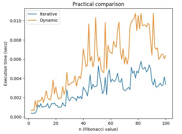

This code uses timeit to get the average execution time for 1000 executions of each algorithm. You can see the difference in execution times for the iterative and dynamic programming approaches when n is large enough. If the problem persists, it may depend on the specifics of your execution environment.

Final Considerations

Let’s see what the asymptotic complexities (big O) are for the proposed algorithms:

Recursive:

• Time complexity: O(2^n)
• The complexity grows exponentially with the value of n.

Iterative:

• Time complexity: O(n)
• The time complexity is linear with respect to the value of n, making the iterative approach more efficient than the recursive one.

Dynamic Programming:

• Time complexity: O(n)
• Dynamic programming exploits the storage of intermediate results to avoid recalculating the same subproblems, thus obtaining a linear complexity with respect to the value of n.

So, in terms of asymptotic efficiency, in the specific example given, it appears that the iterative approach is performing faster than the dynamic programming approach. This can be due to variables such as the specific implementation, execution environment, and computer power.

The O(n) complexity of the iterative approach and the dynamic programming approach indicates that both should have a linear trend as n increases. However, factors such as low-level operations, memory management, and compiler optimizations can affect practical performance.

If you want to more thoroughly examine the differences between the two approaches for your specific input data and execution environment, you may want to do further experiments with larger values of n or on a different system. In any case, asymptotic complexity remains a useful theoretical tool for evaluating the behavior of algorithms on sufficiently large inputs.

Conclusion

In conclusion, choosing the right algorithm is crucial to achieve optimal performance based on the specific needs of the problem. In the context of the Fibonacci series, we looked at three main approaches: recursive, iterative, and dynamic programming. Each of these has its own characteristics and time complexities.

The comparison between the iterative and dynamic programming approaches has shown that, although the asymptotic complexities are both O(n), the practical performance can vary depending on the circumstances. In some cases, the iterative approach may run faster, while in other cases, dynamic programming may show greater efficiency by storing intermediate solutions.

It is important to underline that the choice of the optimal algorithm depends on several factors, including the size of the problem, the complexity of the implementation, the available resources and the peculiarities of the input. I therefore invite experimentation and exploration of optimized solutions, since each context may require a different approach.

Practice and active exploration of different options are key to fully understanding how algorithms perform in a specific context. Analysis of asymptotic complexities provides theoretical guidance, but practical experience and understanding of the problem are crucial to making informed decisions in choosing algorithms.