Algorithms for generating prime numbers in Python

Post Views: 83

Prime number generation is an interesting topic in number theory and has several applications in computer science, cryptography, and other disciplines. There are various algorithms for generating prime numbers in Python, and one of the most common is the Sieve of Eratosthenes algorithm.

[wpda_org_chart tree_id=43 theme_id=50]

The Sieve of Eratosthenes

The Sieve of Eratosthenes algorithm is an efficient method for finding all prime numbers up to a certain limit. Here is a basic implementation in Python:

def eratosthenes_sieve(limit):
    primes = [True] * (limit + 1)
    
    # 0 and 1 are not prime
    primes[0] = primes[1] = False
    
    for number in range(2, int(limit**0.5) + 1):
        if primes[number]:
            # Set multiples of the current number to False
            primes[number**2 : limit + 1 : number] = [False] * len(primes[number**2 : limit + 1 : number])
    
    # Return the prime numbers
    return [number for number in range(2, limit + 1) if primes[number]]

# Example usage
upper_limit = 50
primes_up_to_limit = eratosthenes_sieve(upper_limit)
print(primes_up_to_limit)

Executing you get the following result:

[2, 3, 5, 7, 11, 13, 17, 19, 23, 29, 31, 37, 41, 43, 47]

The Sieve of Eratosthenes algorithm starts with a list of numbers from 2 to n, treats the first number (2) as prime, and then eliminates all its multiples. Next, move on to the next number still marked as first and continue the process.

The Sieve of Eratosthenes has an asymptotic time complexity of $O(n log log n)$ , where $n$ is the upper bound of the primes you are trying to generate. This complexity is very efficient compared to other methods for generating prime numbers and makes the sieve of Eratosthenes a practical choice for most purposes. The $O(n log log n)$ complexity comes from its ability to eliminate multiples of each prime efficiently, reducing the overall number of iterations needed.

The Atkins Sieve and the Sorenson Linear Sieve

There are other algorithms that are more efficient than the Sieve of Eratosthenes for generating prime numbers in certain contexts. Two well-known examples are the Atkins prime number generation algorithm and the Sorenson linear sieve.

Atkins sieve

The Atkins algorithm uses a combination of arithmetic modules and specific selection patterns to identify prime numbers. It has an asymptotic complexity of $O(n / log log n)$ , making it faster than Eratosthenes for some input sizes.

def atkins_sieve(limit):
    is_prime = [False] * (limit + 1)
    sqrt_limit = int(limit**0.5) + 1

    for x in range(1, sqrt_limit):
        for y in range(1, sqrt_limit):
            n = 4 * x**2 + y**2
            if n <= limit and (n % 12 == 1 or n % 12 == 5):
                is_prime[n] = not is_prime[n]

            n = 3 * x**2 + y**2
            if n <= limit and n % 12 == 7:
                is_prime[n] = not is_prime[n]

            n = 3 * x**2 - y**2
            if x > y and n <= limit and n % 12 == 11:
                is_prime[n] = not is_prime[n]

    for n in range(5, sqrt_limit):
        if is_prime[n]:
            for k in range(n**2, limit + 1, n**2):
                is_prime[k] = False

    primes = [2, 3]
    primes.extend([num for num in range(5, limit + 1) if is_prime[num]])
    return primes

limit_superiore_atkins = 50
primi_atkins = atkins_sieve(limit_superiore_atkins)
print(primi_atkins)

Executing you obtain the same result obtained previously:

[2, 3, 5, 7, 11, 13, 17, 19, 23, 29, 31, 37, 41, 43, 47]

Sorenson Linear Sieve

The Sorenson linear sieve is a newer algorithm that has been shown to be efficient for generating prime numbers over specific ranges. It has an asymptotic complexity of $O(n / log n)$ and is especially useful when you need to generate primes on consecutive intervals.

def linear_sorenson_sieve(limit):
    is_prime = [True] * (limit + 1)
    primes = []

    for num in range(2, limit + 1):
        if is_prime[num]:
            primes.append(num)

        for prime in primes:
            if num * prime > limit:
                break
            is_prime[num * prime] = False

            if num % prime == 0:
                break

    return primes

limit_superiore_sorenson = 50
primi_sorenson = linear_sorenson_sieve(limit_superiore_sorenson)
print(primi_sorenson)

Executing you obtain the same result obtained previously:

[2, 3, 5, 7, 11, 13, 17, 19, 23, 29, 31, 37, 41, 43, 47]

It is important to note that the choice of algorithm depends on the specific context and size of the inputs. The sieve of Eratosthenes remains a robust and efficient choice for many cases, but exploring alternative algorithms can be useful in situations where greater optimization for particular dimensions is required.

Both algorithms have different peculiarities and specific optimizations. Efficiency will depend on the specific context in which they are used.

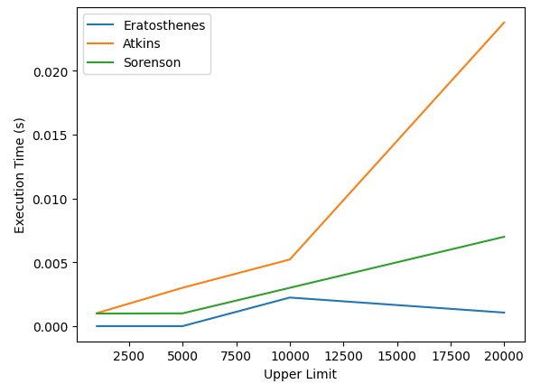
Let’s compare the three algorithms with each other

Let’s see with a practical example how the three algorithms just defined behave in terms of efficiency. Let’s write a test code like the one below:

import time
import matplotlib.pyplot as plt

def time_algorithm(algorithm, limit):
    start_time = time.time()
    algorithm(limit)
    return time.time() - start_time

def eratosthenes_sieve(limit):
    # Implementazione del crivello di Eratostene

def atkins_sieve(limit):
    # Implementazione del crivello di Atkins

def linear_sorenson_sieve(limit):
    # Implementazione del crivello lineare di Sorenson

# Input values
limits = [1000, 5000, 10000, 20000]

# Measure execution times for each algorithm at different bounds
eratosthenes_times = [time_algorithm(eratosthenes_sieve, limit) for limit in limits]
atkins_times = [time_algorithm(atkins_sieve, limit) for limit in limits]
sorenson_times = [time_algorithm(linear_sorenson_sieve, limit) for limit in limits]

# Create the chart
plt.plot(limits, eratosthenes_times, label='Eratosthenes')
plt.plot(limits, atkins_times, label='Atkins')
plt.plot(limits, sorenson_times, label='Sorenson')

# Add labels and legend
plt.xlabel('Upper Limit')
plt.ylabel('Execution Time (s)')
plt.legend()

# Show the graph
plt.show()

By running the code you will obtain the following graph which shows the execution time of the different algorithms to gradually process an ever-increasing number of prime numbers

Probabilistic methods for the generation of prime numbers

Probabilistic methods for generating prime numbers involve the use of algorithms that provide results that are probably correct, but with a minimal probability of error. These algorithms are often preferred in situations where the probability of obtaining an incorrect result can be made extremely low through repeated iterations, and their efficiency can be an advantage compared to deterministic methods.

Here are some probabilistic methods for generating prime numbers:

Miller-Rabin Primality Test: Miller-Rabin primality test is a widely used probabilistic algorithm. It is based on the property that if a composite number is tested as “probably prime”, it is extremely unlikely that it is actually composite. The test can be repeated several times to further reduce the probability of error.
Random Number Generation: A simple method for generating prime numbers is to randomly generate a number, test whether it is odd, and then use a probabilistic primality test such as Miller-Rabin to determine whether it is prime. This process can be repeated until a prime number is found.
Elliptic Curve Approaches: Some algorithms use elliptic curves to generate prime numbers. For example, the “random walk” on an elliptic curve can be used to generate prime numbers probabilistically.
Solovay-Strassen Primality Test: This is another probabilistic test that can be used to determine the primality of a number. It works by comparing the properties of the Jacobi symbol with number theory.
Baillie-Pomerance-Selfridge-Wagstaff (BPSW) primality test: This is another example of a probabilistic primality test. It is known to be probably correct and has been shown to work well in practice, but it is still based on unproven assumptions. The BPSW test is often used in combination with other tests to provide an additional level of confidence in the primality of a number, especially when large numbers used in cryptographic contexts are involved.

It is important to note that these probabilistic methods do not guarantee primality with certainty, but the probability of error can be made extremely small with a sufficient number of iterations or through certain configurations. The adaptability and efficiency of these algorithms make them suitable for many applications, including cryptographic systems where prime numbers are used for cryptographic keys.

Miller-Rabin Primality Test

Let’s see the code for Miller Rabin’s Primality test as an example

import random

def is_probably_prime(n, k=5):
    if n <= 1:
        return False
    if n <= 3:
        return True
    if n % 2 == 0:
        return False

    # Find r and s such that n - 1 = 2^r * s
    r, s = 0, n - 1
    while s % 2 == 0:
        r += 1
        s //= 2

    # Run k iterations of the test
    for _ in range(k):
        a = random.randint(2, n - 2)
        x = pow(a, s, n)  # Calcolo di a^s mod n

        if x == 1 or x == n - 1:
            continue

        for _ in range(r - 1):
            x = pow(x, 2, n)
            if x == n - 1:
                break
        else:
            return False  # n is composed

    return True  #n is probably first

numero_da_testare = 23
ripetizioni_del_test = 5
risultato = is_probably_prime(numero_da_testare, ripetizioni_del_test)
print(f"{numero_da_testare} is probably first: {risultato}")

In this example, the is_probably_prime function takes an integer n and an optional parameter k that represents the number of iterations of the Miller-Rabin test. More iterations reduce the probability of error, but increase execution time.