The HMC5883L magnetometer
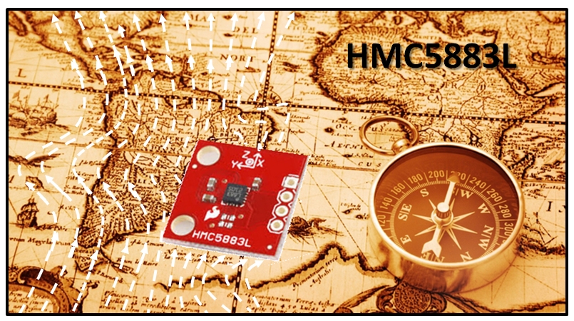
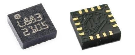
This component (a small chip) HMC5883L, produced by Honeywell, bases its operation on AMR (Anisotropic Magnetoresistive) technology and allows you to be able to measure both the direction and the magnitude of the earth’s magnetic field. This magnetometer HMC5883L has within 3 magneto-resistive sensors arranged on three perpendicular axes (the Cartesian axes x, y and z). Here you can find the component datasheet.
The magnetic field affects these sensors modifying in some way the current flowing through them. Applying a scale to this current, you know the magnetic force (in Gauss) exerted on each sensor.
The component HMC5883L communicates with Arduino through the I2C protocol, a protocol very simple to use.
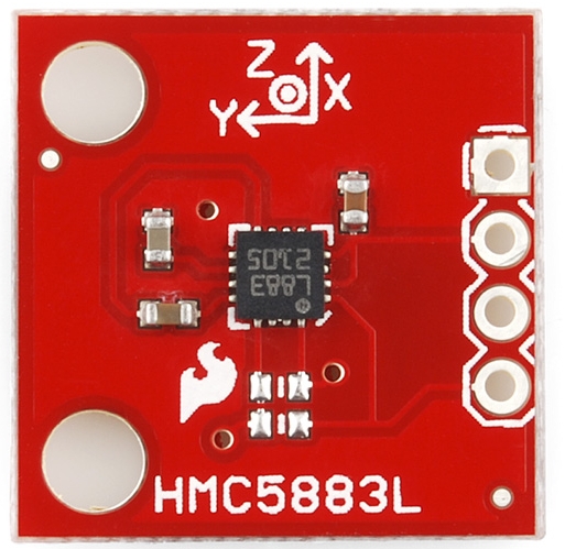
For our example with Arduino, I have bought the breakout board HMC5883L, distributed by Sparkfun (see here), in which the integrated chip is visible in the center (see Fig.2).
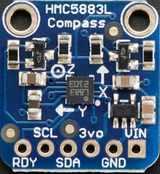
The market offers many other breakout board on which is integrated this chip. A classic example is the breakout board distributed by Adafruit (see here).
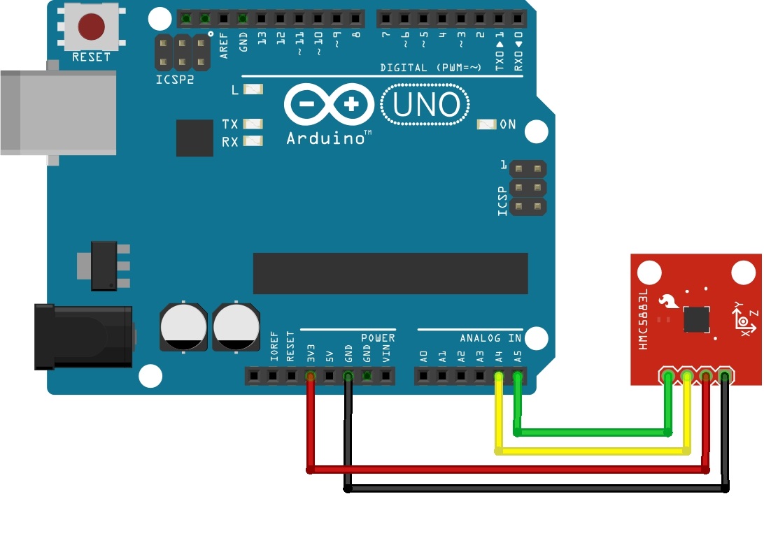
The circuit diagram
- Arduino GND -> HMC5883L GND
- Arduino 3.3V -> HMC5883L Vcc
- Arduino A4(SDA) -> HMC5883L SDA
- Arduino A5(SCL) -> HMC5883L SCL
The HMC5884L library for Arduino
In the internet you can find many libraries programmed specifically for use of this sensor. For the examples discussed in this article I have chosen to use a library downloaded from the website of LoveElectronics some time ago (although now I can not find the site) called just HMC5884L.
Click here to download the library. Once you download the zip file, extract the contents inside the Program Files > Arduino > LIbraries (if you are on Windows), that is a folder named HMC5883L.

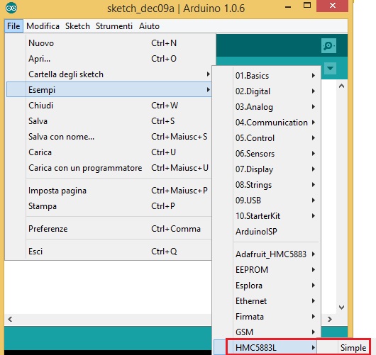
Once you have extracted the contents you start the Arduino IDE. If everything is installed correctly you will find a new example loaded within the IDE (as shown in Fig.5).
May I suggest a site where it presented an excellent tutorial with this library
The best way to learn how to use this library is to use it in simple examples, during which the commands and functions are explained gradually, their operation is that how to use them. For this purpose, in this article you will see two examples. First, you implement a digital compass, then we will use HMC5883L as a real magnetometer, collecting data and then use them in the representation of a vector field through MATLAB.
Let’s create a digital compass
All of you are familiar with this kind of objects. A small cylindrical box with a needle inside of ferrous material that affected by the Earth’s magnetic field, aligns itself according to field lines that run through the surface of the earth, thus indicating the north.
What we want to achieve with Arduino is the creation of a compass that will give us the value 0 ° when the sensor is pointed toward magnetic north, and 180 ° when in fact the sensor is pointing south.
The code that we are using is very common on the Internet and you can find it with endless small variations. I propose it because it is an example very useful to understand how to use this sensor, very simple and suitable as a whole to become familiar with commands of the HMC5883L library.
First you have to import the library HMC5883L.
#include <HMC5883L.h>
Since the HMC5883L board communicates with Arduino through the I2C protocol, you must also import the Wire library (see here for more information).
#include <wire.h>
After including all the required libraries, declare the instance HMC5883L as a global variable.
HMC5883L compass;
Now you can begin to define the content of the two setup() and loop() methods omnipresent in any Arduino sketch.
We begin, as logically, writing the setup() method. First we activate the I2C communication protocol between Arduino and the magnetometer.
void setup() {
    Wire.begin();
Also, since you need to display the values of the magnetometer readings somewhere, you will use the serial communication between Arduino and a PC. Then, specify:
Serial.begin(9600);
Serial.println("Serial started");
After all connections have been initialized, you can now also initialize the magnetometer by defining:
compass = HMC5883L();
The next step will be to configure the sensor according to your needs. First you need to define the gain (response scale) on which to work with the magnetometer.
Serial.println("Setting scale to +/- 1.3Ga");
int error = compass.SetScale(1.3);
if(error != 0)
    Serial.println(compass.GetErrorText(error));
Serial.println("Setting measurement mode to continuous.");
error = compas.SetMeasurementMode(Measurement_Continuous);
if(error != 0)
   Serial.println(compass.GetErrorText(error));
With these lines of code you have just set the gain at 1.3 Ga (end scale), that the measures should be between values of -1.3 and 1.3 Ga.
You can set only some end scale (gain) on the HMC5883L magnetometer, and these are: 0.88, 1.3, 1.9, 2.5, 4.0, 4.7, 5.6 and 8.1 gauss. Needless to say, if your measurements fall within a certain range, try to select a smaller scale can that contains it, as the precision of the measurement taken from your card will be higher.
Now you begin to define the content of the loop() function. The code written in this function will run continuously, and then each time it is performed, a measurement will be made by the sensor.
void loop(){
   MagnetometerRaw raw = compass.ReadRawAxis();
The ReadRawAxis() function returns the value obtained directly from the magnetometer. Thus the values obtained in this way have no reference to the true value of the magnetic field strength, but they are only proportional to it. So if you are interested in the true value of the magnetic field (in gauss) you should not consider this function, but replace it with the ReadScaledAxis() function.
In this case, however, you are interested in simulating the orientation of the magnetic needle of a compass, then the actual values do not interest us. So we can safely use the raw values of reading.
Recall that the magnetometer is able to detect simultaneously the measurements on the three Cartesian axes. To obtain these values, just call the following values belonging to the object variable MagnetometerRaw where they are stored. Here’s an example of how we can get the three values each for each axis (to not be included in the code).
int xAxis = raw.XAxis;
int yAxis = raw.YAxis;
int zAxis = raw.ZAxis;
Instead, if you wanted to use the actual values reported directly in scale (measures in Gauss). (to not be included in the code)
MagnetometerScaled scaled = compass.ReadScaledAxis();
int xAxis = scaled.XAxis;
int yAxis = scaled.YAxis;
int zAxis = scaled.ZAxis;
Now you can define the compass needle inside the loop() function.
float heading = atan2(raw.YAxis, raw.XAxis);
if(heading < 0)
    heading += 2*PI;
since the angle you get from this formula is in radians, convert it to degrees format that is most familiar to you and very readable.
float headingDegrees = heading * 180/M_PI;
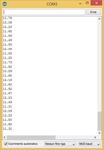
Now you just have to see the value displayed on your PC while it is connected with the Arduino board via serial communication.
Serial.println(headingDegrees);
delay(1000);
I added delay() in order to make a measurement per second (1000 ms), but you may change this measure at your leisure.
Here’s the whole code:
#include <Wire.h>
#include <HMC5883L.h>

HMC5883L compass;

void setup()
{
   Wire.begin();
   Serial.begin(9600);
   compass = HMC5883L();

   Serial.println("Setting scale to +/- 1.3Ga");
   int error = compass.SetScale(1.3);
   if(error != 0)
     Serial.println(compass.GetErrorText(error));

   Serial.println("Setting measurement mode to continuous");
   error = compass.SetMeasurementMode(Measurement_Continuous);
   if(error != 0)
   Serial.println(compass.GetErrorText(error));
}

void loop()
{
   MagnetometerRaw raw = compass.ReadRawAxis();
   float heading = atan2(raw.YAxis, raw.XAxis);
   if(heading < 0)
      heading += 2*PI;
   float headingDegrees = heading * 180/M_PI;
   Serial.println(headingDegrees);
   delay(1000);
}
Now connect the Arduino to the PC and open a serial communication with which you can control your digital compass. Rotate the HMC5883 board until you get the 0 value. If you get 0 you are pointing the north (magnetic).
The magnetic declination
The magnetic field that surrounds the terrestrial globe is neither perfect nor uniform, but is subject to continuous variations in both space and time. This effect is called magnetic declination. In this regard, there is a beautiful animated GIF that I want to propose that presents the variation of the magnetic field during the last four centuries (1590-1990).
As for the digital compass, you can take into account this effect by slightly changing the formula used in the previous example.
First we need to get the value of the magnetic declination of the position in which we are carrying out the measurement. There is a beautiful site in the internet that can provide real-time values of the magnetic declination (www.magnetic-declination.com). This site will give you immediately the magnetic declination of the position in which you are connected. Here’s my example below:
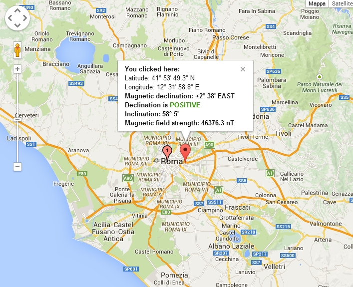
From the box that appears at the center of your map, you will be interested mainly in:
Magnetic declination: +2° 38′ EAST
Now visit WolframAlpha, a beautiful site for the calculation and scientific informationonline. Thanks to it you will convert the value of the magnetic declination in radians. In the input field type
(2° 38') in radians


Thus add the following code within the loop() function :
float declinationAngle = 45.96/1000;
heading += declinationAngle;
This is because I have got a declination EAST, but if the declination is WEST you should write:
heading -= declinationAngle;
And finally…
if(heading <0)
   heading += 2*PI;
if(heading > 2*PI)
   heading -= 2*PI;
float headingDegrees = heading * 180/M_PI;
Another example: let’s visualize the magnetic field on your table
Now we develop another example, in my opinion a bit more fun, though more laborious.
In this example we will take a series of measures on the table next to our computer to display the field lines that pass through it. In the second phase of the example we will introduce a magnet near the area in which we have carried out the previous measures and measures rieffettueremo again. It will be interesting to see the effect that it will introduce the magnet on the field lines that cross our desk.
For the example we are considering will consider only the vector components of the magnetic field on the X and Y axis, viewing the magnetic field that crosses the surface of our table.
First we look at the code for Arduino
#include <Wire.h>
#include <HMC5883L.h>

HMC5883L compass;
int i;
float X_tot, Y_tot, Z_tot;
float X,Y,Z;
void setup()
{
   Wire.begin();
   Serial.begin(9600);
   compass = HMC5883L();

   Serial.println("Setting scale to +/- 1.3Ga");
   int error = compass.SetScale(1.3);
   if(error != 0)
     Serial.println(compass.GetErrorText(error));

   Serial.println("Setting measurement mode to continuous");
   error = compass.SetMeasurementMode(Measurement_Continuous);
   if(error != 0)
     Serial.println(compass.GetErrorText(error));

   i = 0;
   X_tot = 0;
   Y_tot = 0;
   Z_tot = 0;
   X = 0; Y = 0; Z = 0;
}

void loop()
{
   MagnetometerRaw raw = compass.ReadRawAxis();
   if(i<499){
     X_tot += raw.XAxis;
     Y_tot += raw.YAxis;
     Z_tot += raw.ZAxis;
   }else{
     X = X_tot/500;
     Y = Y_tot/500;
     Z = Z_tot/500;
     X_tot = 0; Y_tot = 0; Z_tot = 0;
     i = 0;
     Serial.print(i+":t");
     Serial.print(X);
     Serial.print(" ");
     Serial.print(Y);
     Serial.print(" ");
     Serial.print(Z);
     Serial.println(" ");
     delay(2000);
   }
   i++;
}
As you can see from the code, I used raw measures, but if you want to make a more precise work I recommend you use the scaled measures. I also made sure that the value displayed on the PC serially, is the average of 500 readings. I made several attempts and I saw that this average produces fairly repetitive values. Increasing or decreasing the number of samples to average I get worse results (in your case you can do various tests).
Now we go to the actual measurement.
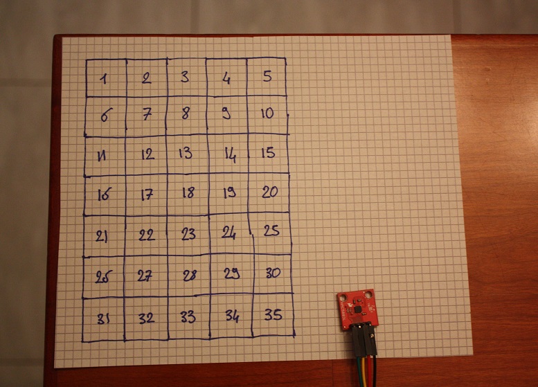
First I took a sheet of squared paper and I drew on it 35 squares each having the same size of the Sparkfun breakout board. I created a matrix of 5×7 squares, and then I numbered each of them in ascending order (see Fig 10).
Then I put the paper on the table, fixing it so that it can not move on it (with tape, or small weights). Once this is done I measured values of the magnetic field on each square, noting both the strength of the magnetic field of the X-axis that Y-axis (NB the values read very often fluctuate, try to see the value that occurs most often)
At the end you will get a table of values. I show you the table of values that I got on my table. They will be those shown in the example.
| X | Y | Z | |
| 1 | -27 | -348 | -386 |
| 2 | -17 | -347 | -388 |
| 3 | 14 | -350 | -389 |
| 4 | 14 | -351 | -390 |
| 5 | -5 | -360 | -393 |
| 6 | -20 | -350 | -377 |
| 7 | -10 | -345 | -380 |
| 8 | 2 | -350 | -387 |
| 9 | 27 | -353 | -390 |
| 10 | 17 | -356 | -394 |
| 11 | -46 | -325 | -368 |
| 12 | -3 | -334 | -380 |
| 13 | 9 | -340 | -386 |
| 14 | -26 | -340 | -388 |
| 15 | -16 | -347 | -400 |
| 16 | 0 | -318 | -232 |
| 17 | 17 | -340 | -368 |
| 18 | 20 | -347 | -385 |
| 19 | 3 | -340 | -401 |
| 20 | 21 | -340 | -408 |
| 21 | -27 | -394 | -308 |
| 22 | -10 | -350 | -378 |
| 23 | -5 | -334 | -398 |
| 24 | -12 | -338 | -404 |
| 25 | -48 | -326 | -423 |
| 26 | -47 | -350 | none |
| 27 | 1 | -346 | none |
| 28 | 1 | -343 | none |
| 29 | 38 | -343 | none |
| 30 | -35 | -330 | none |
| 31 | -80 | -400 | none |
| 32 | 1 | -346 | none |
| 33 | -23 | -342 | none |
| 34 | 15 | -340 | none |
| 35 | -107 | -410 | none |
Once you have all the values, you have to open a session on MATLAB and begin to define a matrix SX and SY containing the measured values respectively for X and Y. These two matrices SX and SY have size 5×7 and the values are inserted into them in the same format that we have on the squared paper, so that the spatial distribution of the measures is respected.
>>SX = [  -27 -17 14 14 -5;
          -20 -10 2 27 17;
          -46 -3 9 -26 -16;
           0 17 20 3 21;
          -27 -10 -5 -12 -48;
          47 1 1 38 -35;
          -80 1 -23 15 -107];
>>SY = [  -348 -347 -350 -351 -360;
        -350 -345 -350 -353 -356;
        -352 -334 -340 -340 -347;
        -318 -340 -347 -340 -340;
        -394 -350 -334 -338 -326;
        -350 -346 -343 -343 -330;
        -400 -346 -342 -340 -410]
also define the spatial arrangement X and Y of each square (measure).
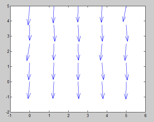
>>x = linspace(0,5,5);
>>y = linspace(0,7,7);
>>[X,Y] = meshgrid(x,y);
>> quiver(X,Y,SX,SY);
and finally you obtain the visualization of the vectors of the magnetic field. The picture is inverted with respect to the picture of the table (the cell 1 is on the bottom left).
Now add a magnet to the left of the sheet to about 7 cm from it and at the center of the sheet.
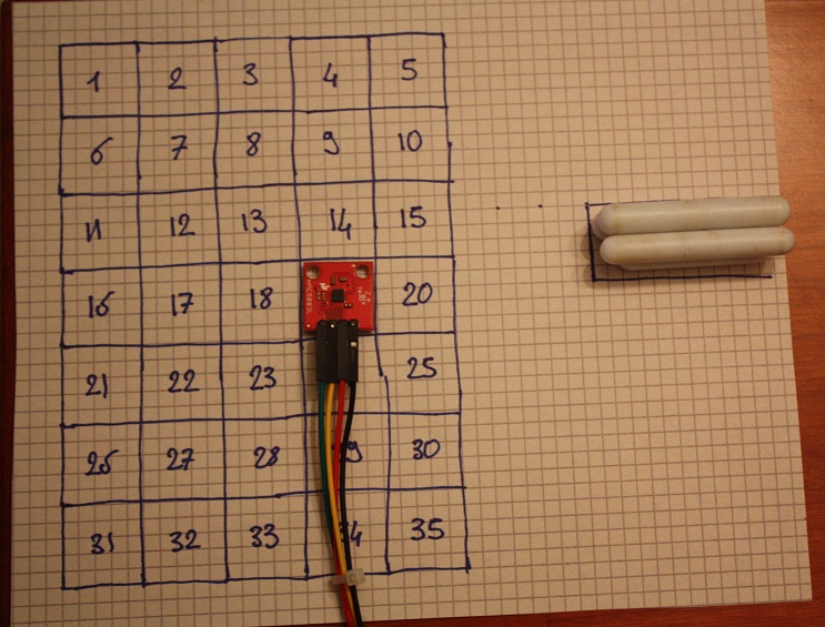
Make again all measures for each square as you did earlier. At the end you’ll get a table similar to the following.
| X | Y | Z | |
| 1 | -109 | -303 | -383 |
| 2 | -108 | -284 | -391 |
| 3 | -130 | -322 | -394 |
| 4 | -174 | -188 | -412 |
| 5 | -244 | -9 | -446 |
| 6 | -124 | -290 | -380 |
| 7 | -158 | -350 | -380 |
| 8 | -185 | -267 | -394 |
| 9 | -329 | -182 | -412 |
| 10 | -756 | -147 | -417 |
| 11 | -125 | -294 | -363 |
| 12 | -127 | -323 | -400 |
| 13 | -199 | -330 | -388 |
| 14 | -403 | -275 | -399 |
| 15 | -975 | -240 | -475 |
| 16 | -73 | -321 | -243 |
| 17 | -105 | -356 | -365 |
| 18 | -178 | -398 | -385 |
| 19 | -406 | -450 | -387 |
| 20 | -778 | -820 | -332 |
| 21 | -98 | -474 | -343 |
| 22 | -106 | -370 | -373 |
| 23 | -154 | -420 | -390 |
| 24 | -157 | -517 | -386 |
| 25 | -390 | -736 | -290 |
| 26 | -85 | -373 | -382 |
| 27 | -93 | -394 | -385 |
| 28 | -89 | -430 | -381 |
| 29 | -121 | -500 | -380 |
| 30 | -113 | -650 | -430 |
| 31 | -74 | -375 | -380 |
| 32 | -76 | -465 | -378 |
| 33 | -38 | -422 | -381 |
| 34 | -65 | -500 | -390 |
| 35 | -160 | -523 | -400 |
Now, again with MATLAB, define two matrices 5×7 VX and VY containing the new measures, and finally re-enter MATLAB commands to obtain the graphical representation.
>>VX = [ -109 -108 -130 -174 -244;
         -124 -158 -185 -329 -756;
         -125 -127 -199 -403 -975;
         -73 -105 -178 -406 -778;
         -98 -106 -154 -157 -390;
         -85 -93 -89 -121 -113;
         -74 -76 -38 -65 -160 ]
>>VY = [ -303 -284 -322 -171 -9;
         -290 -350 -267 -182 -147;
         -294 -323 -330 -275 -240;
         -321 -356 -398 -450 -820;
         -474 -370 -420 -517 -736;
         -373 -394 -430 -500 -650;
         -375 -465 -422 -500 -523 ]
With the hold on command you overlay the new representation with the previous one in order to better visualize the changes in the earth’s magnetic field introduced by the approach of a magnet.
>> quiver(X,Y,SX,SY);
>> hold on
>> quiver(X,Y,VX,VY);
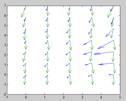
As you can see the effect is quite significant in the vicinity of the right edge and is gradually decreasing with the move away from the magnet.
Conclusions
This small article is just a small introduction to the great potential of this sensor. It would be very interesting to extend the previous example to three dimensions considering the Z-axis. Another good idea would be to monitor the variation in time of the magnetic field.
But this is up to you! See you next article.