This is the second in a series of articles illustrating how to develop a dendrogram, using the D3 JavaScript Library, built on the basis of a particular data structure contained within a JSON file.
Read the article how to make a dendrogram with the D3 Library (Part 1)
In This article first we will develop the JavaScript code that will allow us to view the following tree structure:
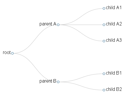
As we said in the previous article, when in a dendrogram we do not take into account the ultrametric distances, we actually have to do with a tree structure.
The following is the code of the Web page that we will save as dendrogram01. html.
<!doctype html>
</html>
<meta charset="utf-8" />
<style>
.node circle {
     fill: #fff;
     stroke: steelblue;
     stroke-width: 1.5px;
}
.node {
     font: 20px sans-serif;
}
.link {
     fill: none;
     stroke: #ccc;
     stroke-width: 1.5px;
}
</style>
<script type="text/javascript" src="http://d3js.org/d3.v3.min.js"></script> <script type="text/javascript">
var width = 600;
var height = 500;
var cluster = d3.layout.cluster()
    .size([height, width-200]);
var diagonal = d3.svg.diagonal()
    .projection (function(d) { return [d.y, d.x];});
var svg = d3.select("body").append("svg")
    .attr("width",width)
    .attr("height",height)
    .append("g")
    .attr("transform","translate(100,0)");
d3.json("dendrogram01.json", function(error, root){
     var nodes = cluster.nodes(root);
     var links = cluster.links(nodes);
     var link = svg.selectAll(".link")
         .data(links)
         .enter().append("path")
         .attr("class","link")
         .attr("d", diagonal);
     var node = svg.selectAll(".node")
         .data(nodes)
         .enter().append("g")
         .attr("class","node")
         .attr("transform", function(d) { return "translate(" + d.y + "," + d.x + ")"; });
     node.append("circle")
         .attr("r", 4.5);
     node.append("text")
         .attr("dx", function(d) { return d.children ? -8 : 8; })
         .attr("dy", 3)
         .style("text-anchor", function(d) { return d.children ? "end" : "start"; })
         .text( function(d){ return d.name;});
});
</script>
If you now open the HTML file within any browser you will get the Dendrogram represented in Fig. 1. Warning: the DENDROGRAM01. json file must be in the same directory as the HTML page, otherwise you will have to correct the path within the D3. JSON () function. Now let’s start analyzing the JavaScript code that we used.
var width = 600;
var height = 500;
With these two variables we define the size of the drawing area within our Web page. We will have an AR 600×500 dedicated to the representation of our dendrogram.
var cluster = d3.layout.cluster()
     .size([height, width-200]);
var diagonal = d3.svg.diagonal()
     .projection (function(d) { return [d.y, d.x];});
First, having decided to work with a tree structure, we will therefore have to manage a whole series of data that will respond to a hierarchical structure. The D3 library gives us a whole series of tools to manage data structures of this type (layouts) that greatly simplify the task. For Dendrograms, the layout we’re going to use is the cluster (D3. Layout. Cluster).
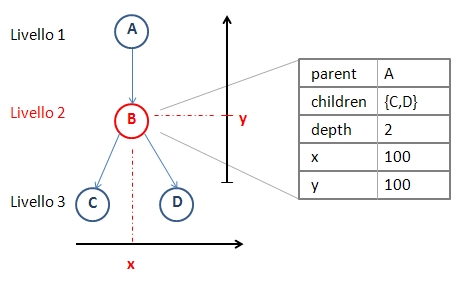
The cluster layout is an object variable with an internal tree structure composed of many object nodes, each of which is characterized by the following attributes:
- Parent: The parent node, is null for the root node.
- Children: The array of child nodes, is null for leaf nodes.
- Depth: The level of the node in the tree.
- X: The x-coordinate of the node.
- Y: the y-coordinate of the node.
Then in the code we define the cluster layout, assigning it a portion (500x400pixel) of the drawing area (500×600).
Another class of objects that we need to properly represent our tree, are the diagonal, that is those graphic elements that allow us to draw the branches (links) that unite the various nodes between them.
The diagonal (D3. svg. Diagonal) are graphical elements that generate a cubic Bezier curve between two points, and these kinds of objects are widely used in the D3 library for all diagrams where there is a need to represent a link between two elements in Separate points in the drawing area.
Bezier curves are curves built through a certain set of parameters (in SVG are expressed through the paths), very used in computer graphics. Depending on the number of parameters passed, you will gradually get more and more complex curves.
The following figures are taken from WikiPedia and represent respectively the construction of quadratic Bezier curves (1 point defined beyond the origin and destination), cubic (2 points defined beyond the origin and destination) and Quartics (3 points defined Beyond the Orifine and the destination).


Once these curves are defined, using the projection () method, we assign the x and Y values of each node (d. x and D. Y).
Once these objects are defined, it’s time to define the code needed to construct the root element
var svg = d3.select("body").append("svg")
     .attr("width",width)
     .attr("height",height)
     .append("g")
     .attr("transform","translate(100,0)");
Now is the time to read and interpret the data contained within the file DENDROGRAM01. JSON (this file was described in the previous article). The iterative anonymous function will start reading from the root element of the data structure (root) that we will pass appropriately to the cluster. nodes () function. This function belongs to the cluster layout, returns an array of object nodes that we will assign to the nodes variable. Soon after, we’ll use this array nodes passing it as an argument to the cluster. Links () function. This other function, which is always part of the cluster layout, calculates the branches of the tree structure by defining an array of objects links, which we will assign to the links variable.
d3.json("dendrogram01.json", function(error, root){
    var nodes = cluster.nodes(root);
    var links = cluster.links(nodes);
With these few lines of code, we built the entire DENDROGRAM data structure (it’s really handy).
Now we can begin to draw the various graphic elements directly. We start from the branches of the Dendrogram. The following lines will draw a path SVG (that is, a Bezier curve) for each link object contained within the links array (the previously generated array when reading the JSON file).
var link = svg.selectAll(".link")
    .data(links)
    .enter().append("path")
    .attr("class","link")
    .attr("d", diagonal);
Now let’s draw the knots. Each node will be represented by a small circle (SVG circle) of 4.5 radius Pizel. Each circle will be drawn in the (x, y) position defined within the object node. In This example (tree structure), the x and Y values of each node are calculated automatically through the cluster. nodes () function.
var node = svg.selectAll(".node")
     .data(nodes)
     .enter().append("g")
     .attr("class","node")
     .attr("transform", function(d) { return "translate(" + d.y + "," + d.x + ")"; });
node.append("circle")
     .attr("r", 4.5);
Now it’s time to add the name of each node, which is also contained within the JSON file.
node.append("text")
     .attr("dx", function(d) { return d.children ? -8 : 8; })
     .attr("dy", 3)
     .style("text-anchor", function(d) { return d.children ? "end" : "start"; })
     .text( function(d){ return d.name;});
And with that we have finished the code of this first example.
In the next article we will realize a real dendrogram, in which the distances of the knots are quantitatively evaluable.