Scatterplots are a straightforward way to visualize the data distribution in a XY plane, especially when we are looking for trends or clusters. But when you have a dataset with a large number of points, many of these data points can overlap. This overalpping effect can make difficult to see any trends or clusters.
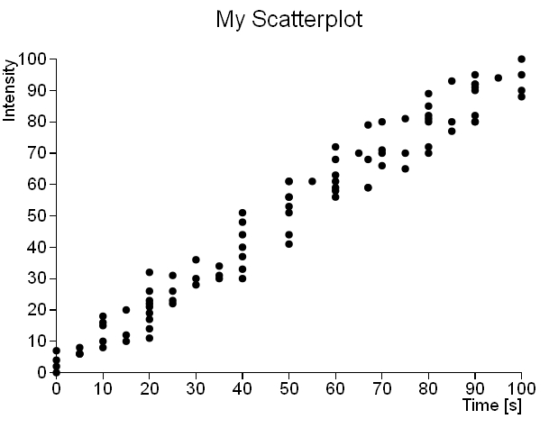
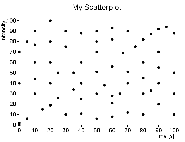
For example, let’s take these two different datasets which are represented in the following scatterplots (see Figures 1 and 2). The first scatterplot unequivocally shows the linear trend underlying the dataset. Instead the second scatterplot apparently shows a uniform distribution of the data points throughout the XY plane (actually there are a lot of overlapping points that are not visible).
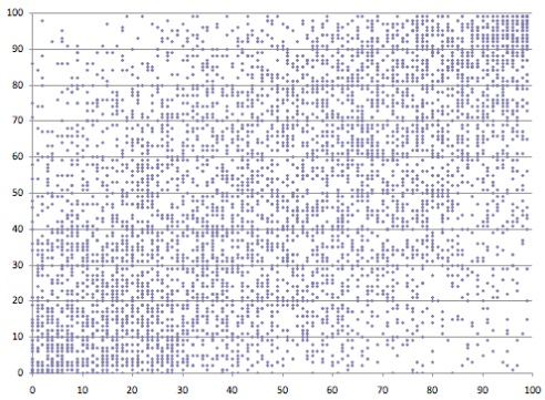
Note: I have used this “sparse” dataset to make easier to understand the concepts covered in this article. The following picture (see Figure 3) shows a more real case.
If you analyze in detail the second dataset, it turns out that multiple data points are occupying the same place in the scatterplot, thereby distorting the visualization of the data distribution on the XY plane. Thus, a scatterplot can only represent point density up to a certain threshold.
In these cases, we need to choose another type of visualization which uses binning methods, in order to plot the point density rather the point themselves. A binned representation is a technique of data aggregation which may reveal patterns not readily apparent in a scatterplot.
Binning
Binning is a technique of data aggregation used for grouping a dataset of N values into less than N discrete groups. In this article we are considering only the case of datasets build up of (x,y) points distributed on a XY plane, but this technique is applicable in other cases. This technique is based on extremely simple concepts.
- the XY plane is uniformly tiled with polygons (squares, rectangles or hexagons).
- the number of points falling in each bin (tile) are counted and stored in a data structure.
- the bins with count > 0 are plotted using a color range (heatmap) or varying their size in proportion to the count.
Note: If we consider the case of monodimensional datasets, the binning technique generates histograms.
Rectangular Binning
The simplest binning method use square tiles, and for most purposes this suffices, taking advantage of its computational simpliticy.

If you are interested to develop charts using the rectangular binnings method, there is a tutorial about this topic showing how to make it using the JavaScript library D3.
Hexagonal binning
This technique was first described in 1987 (D.B.Carr et al. Scatterplot Matrix Techniques for large N, Journal of the American Statistical Association, No.389 pp 424-436). There are many reasons for using hexagons instead of squares for binning a 2D surface as a plane. The most evident is that hexagons are more similar to circle than square. This translates in more efficient data aggregation around the bin center. This can be seen by looking at some particular properties of hexagons and, especially, of the hexagonal tessellation.
- Hexagon is the polygon with the maximum number of sides for a regular tessellation of a 2D plane.
This makes the hexagonal binning the most efficient and compact division of 2D data space.

In fact, although you can create many pattern using two or more types of polygons, this is not possible if you are using the same polygon if this has more than 6 sides. Only triangles, squares and hexagon can create them.
- In an hexagonal binning, adjacent hexagons shares edge borders and not only vertex borders.
Instead in square and triangular binning, triangles and square share only a vertex border with some adjacent.
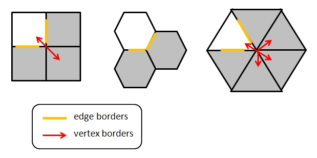
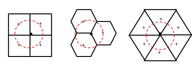
Considering polygons with equal area, the more similar to a circle this polygon is, the closer to the center the border points are (especially vertices).
Thus any point inside a hexagon is closer to the center of any given point in an equal area square or triangle would be. This is because square and triangles have more acute angles.
Sparse Scatterplot in Hexagonal Binning
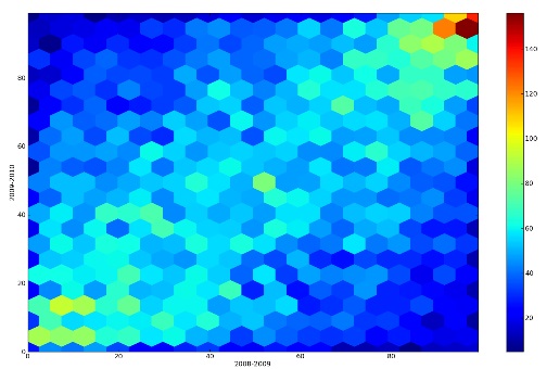
Now that we have an idea of what the hexagonal binning is, let’s submit the dataset which generated a “sparse” scatterplot to a hexagonal binning. This is the result:

I used a range of colors starting from yellow up to a dark red. White bins are the bins where there is no data (count = 0). As we can see in the Figure 8, now a linear trend is visible.
Multivariate Hexagonal Binning
This effect can be further accentuated if we consider the possibility to draw hexagons with size proportional to the count. This can be seen in the next Figure. In this case the variable distribution represented by color value/saturation is the same as that represented by size.
But generally they could be different, that is, for example, the size could represent the standard deviation.

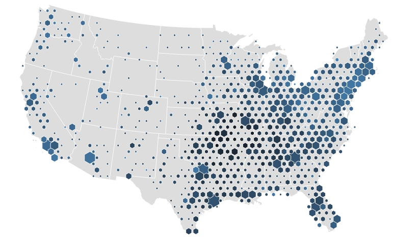
The Choropleth maps
Just in recent months, the hexagonal binning is having a rapid spread in a specific field: cartography. In fact this topic has becoming increasingly popular in many articles and posts where many applications of hexagonal binnings for generating choropleth maps are discussed.
The choropleth maps are thematic maps in which areas are shaded or patterned in proportion to the measurement of the statistical variable being displayed on the map.
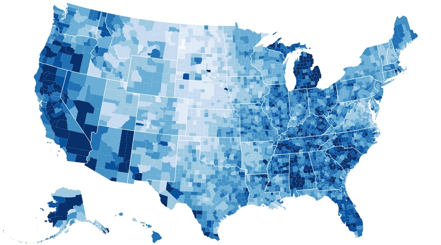
The novelty is using hexagonal bins to represent data on maps. This approach can be a powerful way to deal with cases where there are a large number data points.
References
- C. Stucchio – Don’t use scatterplots
- N. Lewin-Koh – Hexagon Binning: an Overview.
- Hexbins!
- Graham – An introduction to Hexagonal Geometry
Choropleth Maps with D3
- S.Hall – Delimited – Hexbins with D3 and Leaflet Maps
- M. Bostock – Choropleth
- M. Bostock – Bivariate Hexbin Map