Inverse Kinematics

Post Views: 5,213

When we talk about inverse kinematics we mean the set of methodologies that allow to determine the motion of a robot to reach a desired position. But there is no better way to explain what inverse kinematics is than with a practical example …

The 2-link and 2-joint manipulator

Let’s consider the simplest robot model.

Suppose we have a manipulator consisting of two links and two joints bent in the corners $\theta_1 ^ A$ and $\theta_2 ^ A$ , respectively. The effective end will be at a position A defined by the $(x_A, y_A)$ coordinates. This is the starting position.

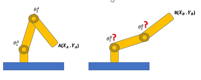
Inverse kinematics - la cinematica inversa

Now, however, the effective end to work will have to move to a new position B having $(x_B, y_B)$ coordinates. What will be the two new angles $\theta_1 ^ B$ and $\theta_2 ^ B$ that the two joints will have to assume in order for the effective end to be correctly in position B ?

This is a classic Inverse kinematics problem.

How to solve ?

In order to solve this problem it will be necessary to use the direct kinematics equations of the manipulator. Since these equations are not linear, finding a solution is certainly not that easy and straightforward. Furthermore, the solution is often not unique. In fact, it is possible to have different combinations of joint angles to obtain the same desired position (x, y). These aspects increase the greater the complexity of the manipulator system under study.

Even the simplest case, that is the case we have considered, that of a manipulator with two links and two joints, presents some difficulties.

not all positions (x, y) are reachable from the effective end and in this case there are no solutions in the equations.
there can be two solutions, corresponding to two different configurations of the manipulator (elbow up and elbow down).

Inverse kinematics - configurazioni di un manipolatore a 2 link elbow up e elbow down

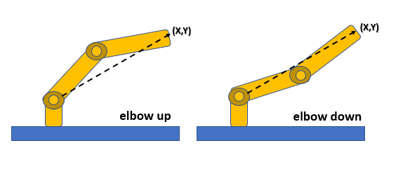
Let’s solve the problem analytically by considering the following diagram:

Inverse kinematics - parametri del manipolatore

The law of cosines can be used to derive the angle θ₂

$cos \theta_2 = \frac { x^2 + y^2 - \alpha_1^2 - \alpha_2^2 }{ 2 \alpha_1 \alpha_2 } = D$

$\theta_2 = cos^{-1} (D)$

An easier way will be to consider instead sin(θ₂).

$sin \theta_2 = \pm \sqrt{ 1 - D^2 }$

And therefore, θ₂ can be derived as

$\theta_2 = tan^{-1} \frac{\pm \sqrt{ 1 - D^2}}{D}$

With this type of analytical approach it is possible to consider both solutions (elbow-up and elbow-down configurations) by choosing the positive and negative signs in the equation.

$\theta_1 = tan^{-1} (\frac{y}{x}) - tan^{-1} (\frac{\alpha_2 sin \theta_2}{\alpha_1 + \alpha_2 cos \theta_2})$

As can be seen from the above equation, we deduce that the angle θ₁ depends on θ₂. This evaluation is plausible since this angle will absolutely depend on which solution it is chosen for θ₂