Matlab is an application that we all know but we do not always have awareness of its potential. In fact, Matlab, in addition to perform the direct numerical calculation in which we are all accustomed to, it also allows us to evaluate analytically (ie, by keeping the parametric expressions) many of these calculations. In fact, thanks to the Symbolic Math Toolbox, Matlab provides us with a set of instructions for the symbolic (or literal) calculation.
Rather than making calculations on known numbers, as you usually do with Matlab, you can make calculations on symbolic expressions. This is useful when you don’t want to immediately compute an answer, or when you have a mathematical formula to work on but you don’t want to process it numerically.
Thus, with Matlab you can perform many mathematical operations analytically:
- derivation and integration
- equation solving
- formula manipulation and simplification
- numerical series (Taylor,..)
- limit calculation
- transform (transform (Fourier, Laplace, etc.)
- vector analysis (jacobian, laplacian,..)
Defining Symbolic Expressions: sym and syms
Symbolic calculation is performed with variables of the class sym (defined by the Symbolic Toolbox). If you need to perform a symbolic calculation with a certain set of variables, you first have to declare these variables as symbolic. This can be done using the sym and syms commands.
Consider the case you want to compute the sine value of an angle θ, with θ = π/2.
>> theta = pi/2;
ans =
           1
Rightly, you get get a numeric value. But sometimes, you need to keep the mathematical expression (in this case a simple sine calculation) in a symbolic format. Thus, you have to declare the angle as a symbolic value using the sym( ) function.
>> x = sym('theta')
x =
      theta
>> sin(x)
ans =
    sin(theta)
This time the expression keeps the theta angle as a parameter.
Generally if you need to define more symbolic variables, for example, to specify the following function
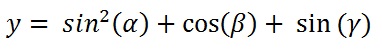
you have to use the syms command followed by three parameters and (optionally) then specifying the type of data (i.e real).
>> syms alpha beta gamma real
>> y = sin(alpha)^2 + cos(beta) + sin(gamma)
ans =
    y = sin(alpha)^2 + cos(beta) + sin(gamma)
When syms is used without any argument, all symbolic values in the workspace will be listed. The commands sym and syms are Matlab’s reserved word. Personally, for simplicity and clarity in the syntax, I prefer to always use the command syms even in the case of a single parameter.
 >> syms theta
>> sin(theta)
ans =
       sin(theta)
Plotting Symbolic Function
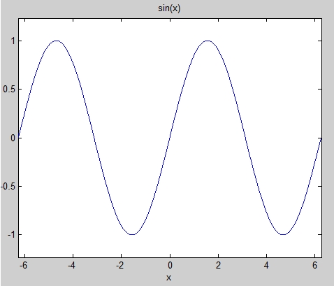
In Matlab you can plot a symbolic function over on a variable by using the ezplot() function. Here is an example:
>> syms x real
>> y = sin(x);
>> ezplot(y);
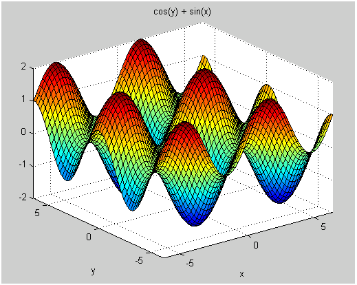
If you prefer to deal with more cool plotting, try the ezsurf() function for the 2D plotting.
>> syms x y real
>> f = sin(x);
>> g = cos(y);
>> ezsurf(f+g);
or more cool!
>> ezsurf('real(atan(x+i*y))');
Equation solving
Another useful case is the possibility to finding the roots of a polynomial. Consider the following symbolic equation:

You can find the roots, that is the x values solving this equation, using the solve() function.
>> syms x a b x
>> y = a*x^2-2*b*x+c;
>> solve(y)
ans =
(b + (b^2 - a*c)^(1/2))/a
(b - (b^2 - a*c)^(1/2))/a
Formula Manipulation and Simplification
Often, when we are working with symbolic expressions, especially with polynomials, we need to expand or simplify them. The expand() function expands a formula where it is possible. For example you can rewrite products of sums as sums of products.
>> syms x a b;
>> f = (x+a)*(x+b)
>> expand(f)
ans =
a*b + a*x + b*x + x^2
The opposite operation to the expansion is the simplification. This is performed by the simplify() function. To see how you can manipulate polynomial expressions, consider as an example a cubic binomial.
First you can expand it
and then if you now simplify the result you get the cubic binomial again.
>> syms x a;
>> f = (x+a)^3
>> g = expand(f)
g =
a^3 + 3*a^2*x + 3*a*x^2 + x^3
>> simplify(g)
(a + x)^3
Derivation and integration
Matlab can also compute many integrals and derivative that you might find in Calculus or many advanced engineering courses. The key functions are int() for integration and diff() for derivation.
Derivative
Let’s consider the following function:

Let’s suppose you want to get the analytical (symbolic) expression of the its derivative. First you have to specify the symbolic variable x and the expression of the function you want to derivate. Then you have to pass the just defined function within the diff() function. In this way, Matlabs returns the analytical expression you need.
>> syms x
>> f = x^3 - cos(x);
>> g = diff(f)
     g = 3*x^2 + sin(x)
If we need to compute the 2nd (or greater) derivative of an equation, we have to specify a second argument in the diff() function: diff(x,n), where n is the order of the derivative. For example, if we want the 2nd derivative of the symbolic function f defined above we have to enter:
>> g = diff(f,2)
     g = 6*x + cos(x)
Partial derivative
So far we have used the diff command with a function which has only one independent variable x. Thus the diff command performed the derivate of the function with respect to x. If there are more than one independent variable in a function, you should specify the variable of derivation as second parameter.
>> diff(f,y)
where y is the variable of derivation. Note that in this case, the command diff(f,y) is equivalent to
For example, if we wish to obtain the derivative of the following function with respect to the variable y:
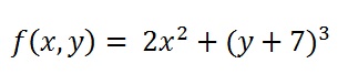
>> syms x y
>> f = 2*x^2 + (y+7)^3;
>> diff(f,y)
ans=
    3*(y + 7)^2
Integrations
In the same way, if you need to get the analytical (symbolic) expression of the indefinite integral, you can use the int() function in a similar way as you done with diff(). Let’s consider the same function you used for the derivation.
>> syms x y
>> f = 2*x^2 + (y+7)^3;
Even here, if the function has more than one parameter, we need to specify the variable of integration as second argument, that in this case is the x variable. Matlab returns:
>> int(f,x)
ans =
     1/3*x^3+(y+5)^3*x
As we can see, we still get a symbolic expression as result. Instead, if you need to compute a definite integration between two values (i.e between 0 and 10)
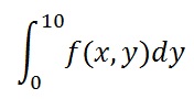
you have to specify other two arguments within the int() function.
 >> int(f,y,0,10)
ans =
    12500+10*x^2
In this case the symbolic expression y has been replaced by numerical values.

Limits
Even the limits can be symbolically computed and the results can sometimes be very interesting. For the calculation of the limits you have to use the limit() function. Just to see the potential of this tool, let’s consider one of the most popular limit:

>> syms x
>> limit(sin(x)/x)
ans =
        1
The limit() function used with only one parameter implicitily considers the case when the default variable approaches 0. Instead the more general case, when the default variable approache to another value, we have to specify it within the limit() function as second argument.
>> syms x
>> limit(sin(x)/x, inf)
ans =
        0
Series and summations
Summations
You can use Matlab to get the summations, when they exist, by using the symsum() function. For example, we can compute the summation of the following series:


>> syms x k
>> s = symsum(1/k^2,1,inf)
s =
      pi^2/6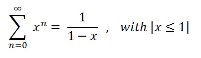
Another example could be the summation of a geometric series:
>> syms x k
>> s = symsum(x^k,k,0,inf)
s =
piecewise([1 <= x, Inf], [abs(x) < 1, -1/(x - 1)])
Taylor series
If you would like to compute the Taylor series of a function, you only need to use the taylor() function passing the symbolic function as argument. For example let’s consider the following function:
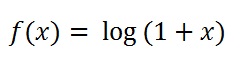
now you can compute the Taylor series:
>> syms x
>> f = taylor(log(1+x))
f =
x^5/5 - x^4/4 + x^3/3 - x^2/2 + x
>> pretty(f)

  5    4    3    2
 x    x    x    x
 -- + -- + -- + -- + x
 5    4    3    2
Notice the result of the pretty() function. This function prints the symbolic output in a format that resembles typeset mathematics. The following Matlab commands will display a plot where the Taylor approximation and the actual function are compared.
>> xd = 1:0.05:5; yd = subs(f,x,xd);
>> ezplot(f, [1, 3]); hold on;
>> plot(xd, yd, 'r-.')
>> title('Taylor approximation vs. actual function');
>> legend('Taylor','Function')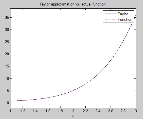
Matrix Symbolic Calculation
Needless to say that the daily bread and butter of all engineers is the calculation of matrices. Even more so when you consider the great potential value to calculate the matrices maintaining long calculations the parameters undefined.
Let’s consider two generic matrices 2×2 with all their elements defined by parameterd. You can refer to them as matrix A and matrix B.
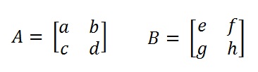
Now, in Matlab, first you have to define 8 symbolic variables corresponding to the elements of the two matrices. Then, you define the two matrices as you have always done with Matlab.
>> syms a b c d e f g h
>> A = [a,b;c,d];
>> B = [e,f;g,h];
Now that you have defined everything you need, let’s see how to add these two matrices. The addition of two parametric matrices generate a further parametric matrix 2×2.
>> C = A + B
C =
[a+e, b+f]
[c+g, d+h]
Similarly, the product of A and B produces a new matrix keeping inside the original parameters.
>> D = A*B
D =
[a*e+b*g, a*f+ b*h]
[c*e+d*g, c*f+d*h]
Of course now you’re wondering – OK, I’m working symbolically and i can see the starting parameters, but now I want to replace the parameters with actual numeric values. Ok. No problem. If we wish to evaluate a specific matrix numerically, we simply assign the numeric values to the appropriate variables, then you can use the command eval to get the a matrix with all the elements as numerical values.
>> a=1;b=2;c=3;d=4;e=5;f=6;e=7;f=8;g=9;h=0;
>> eval(A)
ans =
1 2
3 4
Another common operation on matrices is the inverse matrix. You can obtain the inverse of A using the inv() command as you usually do with numerical matrices, but the result will be expressed symbolically:
>> D = inv(A)
D =
[ d/(a*d-b*c), -b/(a*d-b*c)]
[-c/a*d-b*c),a/[a*d-b*c)]
Again, if you wish to numerically consider the inverse of A, you need to use the eval() command.
>> Dn = eval(inv(A))
Dn =
-2.0000 1.0000
1.5000 -0.5000
All the people, approaching to the robotic world, will soon find out how important it is the symbolic approach to the matrix calculation, especially for the jacobian matrix calculation.
However, even all the others who generally work with Matlab, have now realized the importance of working with mathematical expressions “symbolically”.