When dealing with a set of data describing a population and wanting to perform statistical analyzes, the first characteristics to consider are the mean, the median and the mode. Let’s see in this article what they are and how to calculate them with R. At the end there will be some examples on how to visualize them in a graph, such as histograms and candlestick diagrams.
The median
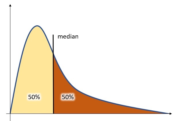
In statistics, the median is that certain value that separates a set of values (population) into two perfectly equal halves. It could be defined as the “middle value”.
In R there is a function that allows us to calculate the median in a very simple way: median(). This function accepts as a parameter a numeric vector containing all the elements of the population.
For example, let’s define the following vector:
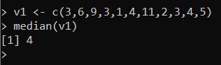
v1 <- c(3,6,9,3,1,4,11,2,3,4,5)Now to calculate the median it will be sufficient to enter:
median(v1)and by executing a value equal to 4 is obtained.
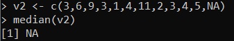
But sometimes it can happen that a vector has no defined values (missing values) and therefore these elements report the value NA. So if we try to re-run the command on the previous array, where there is an undefined value:
v2 <- c(3,6,9,3,1,4,11,2,3,4,5,NA)
median(v2)
unfortunately we will get NA as a result.
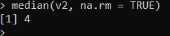
So the defined values need to be handled somehow. In the median () function there is the possibility to pass an additional argument, ba.rm = TRUE, which allows us to exclude all NA values in the incoming vector.
median(x2, na.rm = TRUE)
Now, we get back the same median value we got in the first case, that is 4.
The mode
In statistics, mode is that particular value of a population present in greater numbers (frequency). Therefore it is also possible that a population of data has more than one mode (two values present with the same greater number), or none, as in the case of a uniformly distributed population (all values are present in equal numbers, i.e. they have the same frequency ).
Unfortunately, there is no built-in function in R that can give us the fashion of a population. You will then need to create a function that does this. This simple function only works in case the fashion is unique (i.e. the fashion is unique, otherwise it returns the first fashion it finds).
moda <- function(v) {
   tmp <- unique(v)
   uniqv[which.max(tabulate(match(v, tmp)))]
}
If we use the same element vector used in the previous example:
v1 <- c(3,6,9,3,1,4,11,2,3,4,5)now we will be able to calculate the fashion:
moda(v1)and by executing a value equal to 3 is obtained, which in fact is the value with the highest frequency within the vector.

Now we just have to see how to calculate the population mean
The Mean
The mean is the sum of all the values of a population divided by the number of elements that compose it.
The calculation of the mean is a very common operation, and therefore it could not fail to be present also in R. The mean () function is used to calculate the average of a vector of elements passed as an argument.
Always considering the same vector as the other examples:
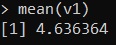
v1 <- c(3,6,9,3,1,4,11,2,3,4,5)The average will be easily calculated by writing:
mean(v1)and executing a value equal to 4.636364 is obtained.
We calculate the median, the mode and the mean on a dataframe
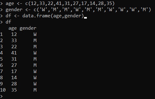
So far we have seen as the most basic example the calculation of the median, the mode and the mean on a vector of elements. Often, when dealing with data to study we have data collected in the form of data frames. To create a dataframe, you first specify the columns as vectors and then merge to form the table (dataframe).
age <- c(12,33,22,41,31,27,17,14,28,35)
gender <- c('W','M','M','W','M','M','W','W','W','M')
df <- data.frame(age, gender)
By executing you get a dataframe with the specified values inside the vectors as columns:
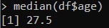
Also in this case it is possible to calculate the median, for the values in the column
median(df$age)and we will find the value of 27.5
Same thing for the mode and the mean
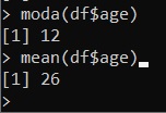
moda(df$age)
mean(df$age)
by executing the commands one at a time, the following values are obtained:
A further step forward will be to calculate the median (or the mean and the mode) based on the group they belong to. If you check the dataframe we have specified, we have a series of ages of individuals in which the gender is specified in the second column (W = woman and M = man).
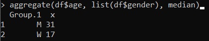
It is possible to calculate two medians based on the sex of the two groups. To do this, combine the aggregate () function with the median function as follows:
aggregate(df$age, list(df$gender), median)In this way, a median is obtained for each gender, 31 for men and 17 for women.
Ssame thing for the calculation of the fashion and the average:
aggregate(df$age, list(df$gender), median)
aggregate(df$age, list(df$gender), mean)
By executing the two commands one at a time, the following values are obtained:

Now that we have seen how to calculate these values it would be a good idea to see how to visualize them in a graph.
Display the median, mean and mode
Now that we’ve seen the median, we’d like to see some ways to visualize it. Generally the median is displayed in population distribution graphs which can be candlestick plots (boxplots) or more generally, histograms.
To help us better in our example representation, we will generate a dataset with a large number of elements. We can use a random generator of elements of a Poisson distribution, the rpois () function. We also enter a precise value as a seed to always get the same random values.
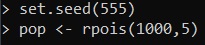
set.seed(555)
pop <- rpois(1000, 5)
At this point we have created a Poisson distribution of 1000 elements having an average value of 5 (lambda).
Let’s calculate the median, as we know how to do:
median(pop)and we will find the value of 5, given in a Poisson distribution the mode is equal to the lambda value passed in the construction of the random distribution.

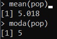
In the same way we can calculate the mean and the mode:
mean(pop)
moda(pop)
By executing the commands one at a time we will get the following values:
Now let’s visualize the Poisson distribution generated in the form of a candlestick diagram. In this case the games are really simple …. in the visualization of a candlestick diagram the median is already highlighted by a black line.
boxplot(pop)In fact, in correspondence with the value 5 we will have a marked horizontal line.

But if we wanted to add a row at the mean, then we will have to add:
boxplot(pop)
abline(h= mode(pop2), col = "blue", lwd=3)
As for the display of the histograms, we will have to add a line corresponding to the median, and we will mark it with the blue color. With the abline () function you can draw a line directly above the histogram.
hist(pop)
abline(v = median(pop), col = "blue", lwd = 3)
In this case mean, mode and median would overlap in the visualization, but in other cases nothing prevents you from adding other lines in their correspondence using different colors.