In the vast landscape of problem-solving algorithms, two main approaches emerge as distinct but complementary methods: Backtracking and Brute Force. Both are used to solve computational problems by exhaustively searching for solutions, but their strategies differ significantly.
In this article, we will examine different dimensions of the two approaches, from computational complexity to their practical application. Through concrete examples and case studies, we will highlight the situations in which Backtracking excels over Brute Force and vice versa. We will also highlight the importance of proper implementation and time complexity considerations.
[wpda_org_chart tree_id=44 theme_id=50]
Backtracking and Brute Force: two approaches compared
Backtracking: The Intelligent Search
Backtracking is a strategy that is based on exhaustive research, but with the addition of an intelligent component. It explores possibilities recursively, making choices and reversing those choices when it recognizes that a partial solution cannot lead to a complete solution. This technique is particularly suitable for complex decision problems, where many unpromising solutions can be eliminated.
Brute Force: The Direct Approach
On the other side of the spectrum, Brute Force is a direct and exhaustive approach that examines all possible solutions one after the other, without pruning strategies or eliminating suboptimal solutions. Although it may be less efficient on complex problems, Brute Force is often used when the problem size is limited or when optimization strategies cannot be applied.
What is Backtracking?
Backtracking is a problem-solving technique that relies on exhaustively searching for all possible solutions to a given problem. In essence, backtracking explores all the possibilities of a solution, and when it realizes that the partial solution it is examining cannot lead to a complete solution, it “backtracks” to the previous decision and resumes exploration from there.
The backtracking technique follows a recursive structure, and its pseudocode can be represented in a general way as follows:
def backtrack(partial_solution, other_parameters):
     if partial_solution is complete:
         # Add partial_solution to solution list
     else:
         for choice in possible_choices:
             if choice is valid:
                 # Make a choice
                 update partial_solution
                 # Recursive call
                 backtrack(partial_solution, other_parameters)
                 # Cancel choice (backtrack)
                 restore partial_solution
The N Queens Problem
This approach is particularly useful for solving decision problems, such as the N queens problem, the traveling salesman problem and many others.
Let’s implement a simple backtracking example to solve the N queens problem. In this problem, the goal is to place N queens on an N x N board so that no queen threatens another.
def is_safe(board, row, col, n):
    # Check if it is safe to place a queen in this position
    for i in range(row):
        if board[i][col] == 1:
            return False
        if col - i >= 0 and board[row - i][col - i] == 1:
            return False
        if col + i < n and board[row - i][col + i] == 1:
            return False
    return True

def solve_n_queens_util(board, row, n, solutions):
    if row == n:
        # We have found a complete solution
        solutions.append([row[:] for row in board])
        return
    for col in range(n):
        if is_safe(board, row, col, n):
            # Make a choice
            board[row][col] = 1
            # Recursive call
            solve_n_queens_util(board, row + 1, n, solutions)
            # Cancel choice (backtrack)
            board[row][col] = 0

def solve_n_queens(n):
    board = [[0] * n for _ in range(n)]
    solutions = []
    solve_n_queens_util(board, 0, n, solutions)
    return solutions

# Example of use
n = 4
solutions = solve_n_queens(n)
for solution in solutions:
    print(solution)
In this example, solve_n_queens will return a list of all possible arrangements of the N queens on the board. The is_safe function checks whether it is safe to place a queen in a certain position. The solve_n_queens_util function is a recursive helper function that explores all possible solutions. Executing you get the following result:
[[0, 1, 0, 0], [0, 0, 1, 0], [1, 0, 0, 0], [0, 0, 0, 1]]
[[0, 1, 0, 0], [0, 0, 0, 1], [1, 0, 0, 0], [0, 0, 1, 0]]
[[0, 0, 1, 0], [1, 0, 0, 0], [0, 0, 0, 1], [0, 1, 0, 0]]
[[0, 0, 1, 0], [0, 1, 0, 0], [0, 0, 0, 1], [1, 0, 0, 0]]
This is just one example of how backtracking can be used to solve a specific problem. The key is to tailor the overall backtracking structure to the specific problem you are addressing.
Backtracking vs Brute Force
Backtracking and brute force are two approaches to solving computational problems comprehensively, but they have significant differences in how they approach finding solutions.
Brute Force
Brute force is a direct and exhaustive approach to solving a problem, in which all possible solutions are examined one after another until the correct one is found. This approach can be inefficient on complex problems, as it examines all possible combinations, without any strategy for pruning or eliminating solutions that cannot lead to an optimal solution.
For example, consider a problem where you need to find the maximum sum of a sub-sequence in an array. Brute force would examine all possible sub-sequences and compare the sums, without considering any structural properties of the problem.
def max_subarray_sum_bruteforce(arr):
    n = len(arr)
    max_sum = float('-inf')
    for i in range(n):
        for j in range(i, n):
            current_sum = sum(arr[i:j+1])
            max_sum = max(max_sum, current_sum)
    return max_sum
This approach can be inefficient for problems with large search spaces.
Backtracking
Backtracking is an approach based on the exhaustive search for solutions, but with the addition of a pruning strategy. It explores solutions recursively, making choices and seeing if they lead to an acceptable solution. If it turns out that a particular choice cannot lead to a valid solution, backtracking “backtracks” and reverses the choice, exploring other possibilities.
In the previous paragraph, we saw an example of backtracking by solving the N queens problem. This approach focuses on incrementally generating solutions, making choices and reversing choices when necessary.
Backtracking is often more efficient than brute force for problems where there are many possible choices and some of them can be intelligently eliminated. However, time complexity can still be high in certain cases.
In conclusion, while brute force examines all possibilities without pruning strategies, backtracking adds a level of intelligence to the search by only exploring relevant possibilities, thus reducing computational time. Both approaches have their uses depending on the specific problem you are addressing.
The Traveling Salesman Problem
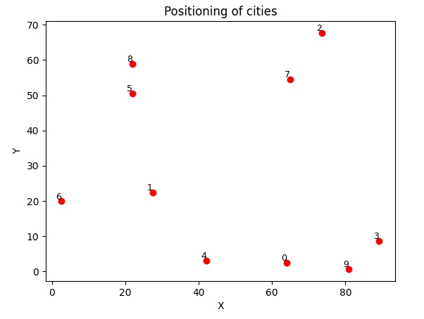
To better see the difference between the Brute Force approach and the Backtracking technique, we will apply a practical example: the Traveling Salesman Problem (TSP), which involves the search for the shortest route that passes through all the data points exactly once.
In this example, we will implement a brute force solution and a backtracking solution to solve the TSP. Next, we will use the matplotlib library to visualize the efficiency differences between the two approaches. We first generate a set of cities randomly arranged in a coordinate space (X.Y).
import random
import matplotlib.pyplot as plt

def distance(city1, city2):
    return ((city1[0] - city2[0]) ** 2 + (city1[1] - city2[1]) ** 2) ** 0.5

def plot_cities(cities):
    x, y = zip(*cities)
    plt.scatter(x, y, c='red', marker='o')
    for i, (xi, yi) in enumerate(cities):
        plt.text(xi, yi, str(i), fontsize=9, ha='right', va='bottom')
    plt.xlabel('X')
    plt.ylabel('Y')
    plt.title('Positioning of cities')
    plt.show()

# Generate random cities for testing
def generate_random_cities(num_cities):
    random.seed(42)
    cities = [(random.uniform(0, 100), random.uniform(0, 100)) for _ in range(num_cities)]
    return cities

# Cities display
num_cities = 10
cities = generate_random_cities(num_cities)
plot_cities(cities)
By executing this we will obtain the graphic representation of the cities arranged on a Cartesian plane
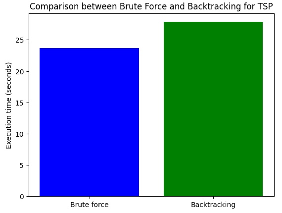
Now we solve the traveling salesman problem using both brute force and backtracking, and finally, we will show a comparative graph of the time taken by the two approaches. Times may vary depending on the random configuration of the cities and the computational power of the system in use.
The calculation must provide us with the shortest route that the traveling salesman will have to take to visit all the cities shown in the graph above. For this calculation we will apply the two different approaches providing two different functions.
Brute Force (tsp_bruteforce)
def tsp_bruteforce(cities):
    start_time = time.time()
    shortest_path = None
    shortest_distance = float('inf')

    for perm in itertools.permutations(range(len(cities))):
        current_distance = total_distance(perm, cities)
        if current_distance < shortest_distance:
            shortest_distance = current_distance
            shortest_path = perm

    elapsed_time = time.time() - start_time
return shortest_path, shortest_distance, elapsed_time- Initialization: The tsp_bruteforce function begins by measuring the start time (start_time) and initializes the shortest_path and shortest_distance variables to keep track of the shortest solution and its distance.
- Permutations: Using itertools.permutations, all possible permutations of city indices are generated. Each permutation represents a possible path to examine.
- Distance Calculation: For each permutation, the total distance of the route is calculated using the total_distance function.
- Best Solution Update: If the calculated distance is less than the current distance of the best solution (shortest_distance), the best solution is updated.
- Time Measurement: At the end of the process, the total time spent is calculated.
Backtracking (tsp_backtracking)
def tsp_backtracking(cities):
    start_time = time.time()

    def backtrack(path):
        if len(path) == len(cities):
            nonlocal shortest_path, shortest_distance
            current_distance = total_distance(path, cities)
            if current_distance < shortest_distance:
                shortest_distance = current_distance
                shortest_path = path
        else:
            for i in range(len(cities)):
                if i not in path:
                    backtrack(path + [i])

    shortest_path = None
    shortest_distance = float('inf')
    backtrack([])

    elapsed_time = time.time() - start_time
return shortest_path, shortest_distance, elapsed_time- Initialization: The tsp_backtracking function begins by measuring the start time (start_time) and initializes the shortest_path and shortest_distance variables.
- Recursive Backtrack Function: The backtrack function is a recursive function that explores all possible permutations of paths. If the length of the current route is equal to the number of cities, the total distance is calculated and the best solution is updated if necessary. Otherwise, for each city not yet included in the route, the function is called recursively by adding the city to the route.
- Backtrack Initialization: The main function tsp_backtracking begins the backtracking process by calling backtrack([]), indicating that the initial path is empty.
- Time Measurement: At the end of the process, the total time spent is calculated.
Backtracking vs Brute Force
Now let’s write the entire code that will calculate the shortest path with both approaches and then we will compare the results obtained and the time taken.
import itertools
import time
import matplotlib.pyplot as plt

def total_distance(path, cities):
    total_dist = 0
    for i in range(len(path) - 1):
        total_dist += distance(cities[path[i]], cities[path[i + 1]])
    return total_dist

# Brute Force Solution for TSP
def tsp_bruteforce(cities):
    start_time = time.time()
    shortest_path = None
    shortest_distance = float('inf')

    for perm in itertools.permutations(range(len(cities))):
        current_distance = total_distance(perm, cities)
        if current_distance < shortest_distance:
            shortest_distance = current_distance
            shortest_path = perm

    elapsed_time = time.time() - start_time
    return shortest_path, shortest_distance, elapsed_time

# Backtracking solution for the TSP
def tsp_backtracking(cities):
    start_time = time.time()

    def backtrack(path):
        if len(path) == len(cities):
            nonlocal shortest_path, shortest_distance
            current_distance = total_distance(path, cities)
            if current_distance < shortest_distance:
                shortest_distance = current_distance
                shortest_path = path
        else:
            for i in range(len(cities)):
                if i not in path:
                    backtrack(path + [i])

    shortest_path = None
    shortest_distance = float('inf')
    backtrack([])

    elapsed_time = time.time() - start_time
    return shortest_path, shortest_distance, elapsed_time

# Running the solutions
bruteforce_result = tsp_bruteforce(cities)
backtracking_result = tsp_backtracking(cities)

# Printing of results
print("Brute force:")
print("Shortest route:", bruteforce_result[0])
print("Minimum distance:", bruteforce_result[1])
print("Execution time (seconds):", bruteforce_result[2])

print("\nBacktracking:")
print("Shortest route:", backtracking_result[0])
print("Minimum distance:", backtracking_result[1])
print("Execution time (seconds):", backtracking_result[2])

# Creation of the comparison graph
labels = ['Brute force', 'Backtracking']
times = [bruteforce_result[2], backtracking_result[2]]
plt.bar(labels, times, color=['blue', 'green'])
plt.ylabel('Execution time (seconds)')
plt.title('Comparison between Brute Force and Backtracking for TSP')
plt.show()
This will take several seconds (almost a minute) to run. At the end of the calculation the following results will be displayed:
Brute force:
Shortest route: (2, 7, 8, 5, 6, 1, 4, 0, 9, 3)
Minimum distance: 203.1584418265072
Execution time (seconds): 23.648714065551758

Backtracking:
Shortest route: [2, 7, 8, 5, 6, 1, 4, 0, 9, 3]
Minimum distance: 203.1584418265072
Execution time (seconds): 27.852330446243286
The result is interesting. In this case, the Brute Force approach would be more efficient than Backtracking, taking a few seconds less to calculate.
