
A Decision Tree is a machine learning model that represents a series of logical decisions made based on attribute values. It is a tree structure which is used to make decisions or make predictions from the input data.
[wpda_org_chart tree_id=22 theme_id=50]
Decision Trees
A decision tree consists of nodes and branches. Nodes represent decisions or tests on an attribute, while branches represent the possible consequences of a decision or test. Decision trees are used for both classification and regression problems.
Here’s how the process of creating a Decision Tree works:
- Attribute selection: The decision tree building algorithm chooses the best attribute to use as the root node. This choice is made based on criteria such as entropy, information gain or Gini impurity. The chosen attribute is used to divide the dataset into smaller subsets.
- Data Breakdown: The data is broken down based on the values of the chosen attribute. Each attribute value generates a branch in the tree, and the data is assigned to the corresponding branches.
- Iteration: The process of selecting the attribute and splitting the data is repeated for each subset of data in each internal node. This process continues until a stopping criterion is met, such as a maximum tree depth or a minimum number of samples in a node.
- Leaf Nodes: Once the splitting process reaches the leaf nodes, i.e. the final nodes of the tree, classification labels (in the case of a classification problem) or prediction values (in the case of a regression problem) are assigned.

If you want to delve deeper into the topic and discover more about the world of Data Science with Python, I recommend you read my book:
Fabio Nelli
The advantages of decision trees include ease of interpretation, as decisions are intuitively represented as logical flows, and the ability to handle both numerical and categorical data. However, decision trees can be prone to overfitting, especially when they are deep and complex.
Decision trees can be further improved using techniques such as pruning, which reduces the complexity of the tree to improve generalization, and ensemble learning, where multiple decision trees are combined to form stronger models, such as:
- Random Forest
- Gradient Boosting.

IN-DEPTH ARTICLE

There are also further more complex algorithmic models specialized for Decision Trees such as:
- CART

IN-DEPTH ARTICLE
A bit of history
Decision trees have a long and interesting history in machine learning and artificial intelligence. Their evolution has led to the development of more advanced techniques, such as Random Forests and Gradient Boosting. Here is an overview of the history of decision trees in machine learning:
1960s: The idea behind decision trees has roots in the 1960s. The concept of “decision programs” was introduced by Hunt, Marin and Stone in 1966. The goal was to create algorithms that could learn how to make decisions through data-driven logical rules.
1970s: In the 1970s, the concept of decision trees was further developed by Michie and Chambers. They introduced the idea of creating decision trees that could be used to make decisions about classification problems.
1980s: In the 1980s, the concept of decision trees continued to evolve as new machine learning techniques were introduced. ID3 (Iterative Dichotomiser 3), developed by Ross Quinlan in 1986, is one of the first machine learning algorithms based on decision trees. ID3 used the concept of information gain to select the best attributes for splitting.
1990s: In the 1990s, the approach to decision trees was further improved with the introduction of new algorithms and techniques. C4.5, introduced by Ross Quinlan in 1993, improved and extended ID3, allowing you to handle numeric and missing attributes and introducing tree pruning to improve generalization.
2000s and beyond: In the 2000s, interest in decision trees increased further. Algorithms such as CART (Classification and Regression Trees) have been developed, which can be used for both classification and regression problems. Furthermore, ensemble learning techniques based on decision trees have been introduced, such as Random Forests (2001) by Leo Breiman and Gradient Boosting (2001) by Jerome Friedman.
Today, decision trees and their variants are widely used in machine learning and data science. They are valued for their ease of interpretation, ability to handle heterogeneous data, and ability to handle both classification and regression problems. Decision trees are often combined into ensemble methods such as Random Forests and Gradient Boosting to further improve model performance.

Suggested book:
Using Decision Trees with scikit-learn
Decision Trees can be used for two Machine Learning problems:
- Classification
- Regression
In Python, you can use the scikit-learn library to build and train decision trees using the DecisionTreeClassifier classes for classification and DecisionTreeRegressor for regression.
Classification with Decision Trees with scikit-learn
Here is an example of how you can use scikit-learn to create and train a Decision Tree Classifier using the Breast Cancer Wisconsin dataset.
Step 1: Import the necessary libraries
from sklearn.datasets import load_breast_cancer
from sklearn.model_selection import train_test_split
from sklearn.tree import DecisionTreeClassifier
from sklearn.metrics import accuracy_score
In this section, we are importing the libraries needed to build and train the Decision Tree Classifier.
Step 2: Load the dataset and split the data
#Load the Breast Cancer Wisconsin dataset as an example
breast_cancer = load_breast_cancer()
X = breast_cancer.data
y = breast_cancer.target

# Divide the dataset into training and test sets<code>
X_train, X_test, y_train, y_test = train_test_split(X, y, test_size=0.2, random_state=42)
Here we are loading the Breast Cancer Wisconsin dataset using the load_breast_cancer() function and splitting the data into training and test sets using the train_test_split() function.
Step 3: Create and train the Decision Tree classifier
# Create the Decision Tree classifier
clf = DecisionTreeClassifier(random_state=42)

# Train the classifier on the training set
clf.fit(X_train, y_train)
In this step, we are creating a DecisionTreeClassifier object and training it on the training set using the fit() method.
Step 4: Make predictions and calculate accuracy
# Make predictions on the test set<code>
predictions = clf.predict(X_test)

# Calculate the accuracy of forecasts<code>
accuracy = accuracy_score(y_test, predictions)
print("Accuracy:", accuracy)
In this step, we are making predictions on the test set using the predict() method of the trained classifier and then calculating the accuracy of the predictions using the accuracy_score() function. By running the code you get the accuracy value
Accuracy: 0.9473684210526315Now we can consider the idea of adding some useful visualizations to understand the validity or otherwise of the model we have just used.
from sklearn.metrics import confusion_matrix
import seaborn as sns
import matplotlib.pyplot as plt
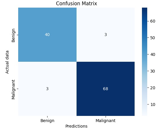
cm = confusion_matrix(y_test, predictions)
sns.heatmap(cm, annot=True, fmt='g', cmap='Blues', xticklabels=['Benigno', 'Maligno'], yticklabels=['Benigno', 'Maligno'])
plt.xlabel('Predizioni')
plt.ylabel('Valori Veri')
plt.title('Matrice di Confusione')
plt.show()Running gives you a confusion matrix. This graph displays the number of true positives, false positives, true negatives and false negatives, giving you a more detailed overview of your model’s performance.
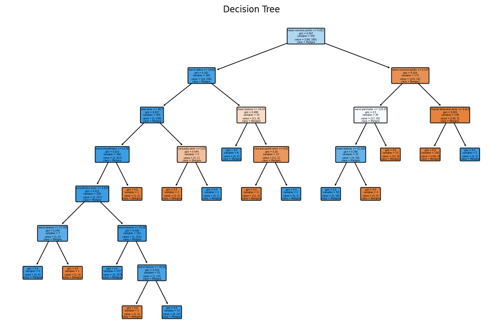
Now, the next graph will aim to visualize the structure of the decision tree.
from sklearn.tree import plot_tree

plt.figure(figsize=(12, 8))
plot_tree(clf, filled=True, feature_names=breast_cancer.feature_names, class_names=['Benigno', 'Maligno'], rounded=True)
plt.title('Decision Tree')
plt.show()
Running the code gives you the following graph depicting the entire decision tree, helping you understand the decisions made by the model. It can be especially useful if the tree is not too large.
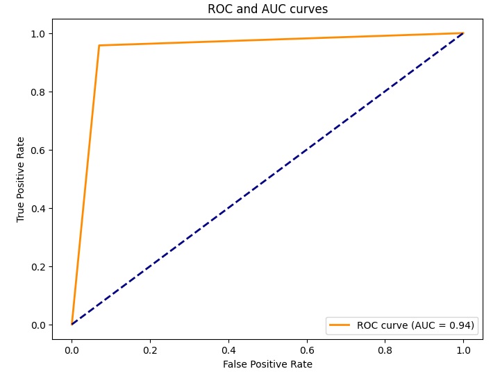
Let’s move on with our visualizations of the Decision Tree model. This time we will use an ROC curve.
from sklearn.metrics import roc_curve, auc

probas = clf.predict_proba(X_test)[:, 1]
fpr, tpr, thresholds = roc_curve(y_test, probas)
roc_auc = auc(fpr, tpr)

plt.figure(figsize=(8, 6))
plt.plot(fpr, tpr, color='darkorange', lw=2, label='ROC curve (AUC = {:.2f})'.format(roc_auc))
plt.plot([0, 1], [0, 1], color='navy', lw=2, linestyle='--')
plt.xlabel('False Positive Rate')
plt.ylabel('True Positive Rate')
plt.title('ROC and AUC curves')
plt.legend(loc='lower right')
plt.show()
By running the code you obtain the ROC curve chart of the model used. This ROC curve displays the trade-off between false positive rate and true positive rate, and the area under the curve (AUC) measures the overall performance of the model.
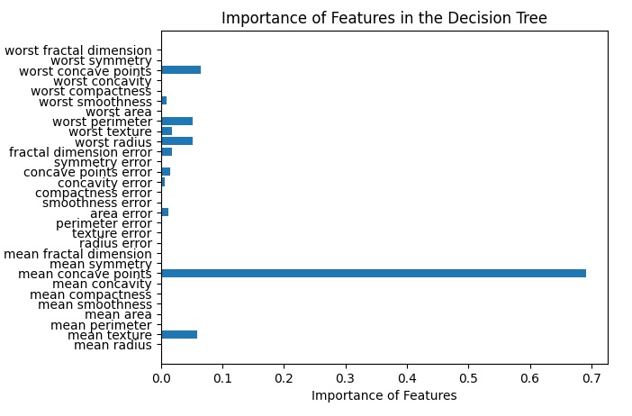
Finally we can analyze the importance of the features to establish how these individually play into the validity of the model used.
feature_importances = clf.feature_importances_
plt.barh(range(len(feature_importances)), feature_importances, align='center')
plt.yticks(range(len(breast_cancer.feature_names)), breast_cancer.feature_names)
plt.xlabel('Importance of Features')
plt.title('Importance of Features in the Decision Tree')
plt.show()
By running this code snippet you get the bar diagram where the weight of each feature in the model statement is depicted.
These steps combined form a complete example of how to use scikit-learn to create and train a Decision Tree Classifier for a classification problem. You can further customize the model using the Decision Tree Classifier hyperparameters to tailor it to your needs.
If you want to delve deeper into the topic and discover more about the world of Data Science with Python, I recommend you read my book:
Fabio Nelli
Decision Tree Regression with scikit-learn
Here is an example of how you can use scikit-learn to create and train a Decision Tree Regressor using the Boston Housing dataset:
Step 1: Import the necessary libraries
from sklearn.datasets import fetch_california_housing
from sklearn.model_selection import train_test_split
from sklearn.tree import DecisionTreeRegressor
from sklearn.metrics import mean_squared_error
In this section, we are importing the libraries needed to build and train the Decision Tree Regressor.
Step 2: Load the dataset and split the data
# Upload the California Housing dataset as an example
housing = fetch_california_housing()
X = housing.data
y = housing.target

# Divide the dataset into training and test sets
X_train, X_test, y_train, y_test = train_test_split(X, y, test_size=0.2, random_state=42)
Here we are loading the California Housing dataset using the fetch_california_housing() function and splitting the data into training and test sets using the train_test_split() function.
Step 3: Create and train the Decision Tree regressor
# Create the Decision Tree regressor
reg = DecisionTreeRegressor(random_state=42)

# Train the regressor on the training set
reg.fit(X_train, y_train)
In this step, we are creating a DecisionTreeRegressor object and training it on the training set using the fit() method.
Step 4: Make predictions and calculate the mean squared error
#Make predictions on the test set
predictions = reg.predict(X_test)

# Calculate the root mean squared error of the predictions
mse = mean_squared_error(y_test, predictions)
print("Mean Squared Error:", mse)
In this step, we are making predictions on the test set using the trained regressor’s predict() method and then calculating the mean squared error of the predictions using the mean_squared_error() function.
Running the above code will give you the MSE value of the predictions made by the model.
Mean Squared Error: 0.495235205629094Also in this case, as for the classification problem, we will be able to use visualizations to evaluate the validity of the model used. In this case we will use different visualizations since we have a regression problem.
import matplotlib.pyplot as plt

plt.scatter(y_test, predictions)
plt.xlabel('Actual Values')
plt.ylabel('Predictions')
plt.title('Comparison between Actual Values and Forecasts')
plt.show()
Running the code will give you a scatterplot showing the relationship between the actual values and the model predictions. Ideally, the dots should align with the diagonal line, indicating a good forecast.

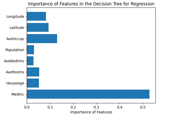
Another visualization is feature importance where the relative importance of each feature in the decision making process of the regression model is shown.
import numpy as np

feature_importances = reg.feature_importances_
plt.barh(range(len(feature_importances)), feature_importances, align='center')
plt.yticks(np.arange(len(housing.feature_names)), housing.feature_names)
plt.xlabel('Importance of Features')
plt.title('Importance of Features in the Decision Tree for Regression')
plt.show()
Another visualization is the error distribution with a histogram showing how the errors are distributed between the model predictions and the actual values.
errors = y_test - predictions
plt.hist(errors, bins=30, edgecolor='black')
plt.xlabel('Errors')
plt.ylabel('Frequency')
plt.title('Distribution of Errors in Decision Tree Regression')
plt.show()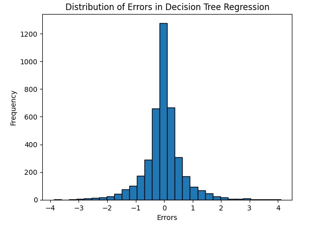
These steps combined form a complete example of how to use scikit-learn to create and train a Decision Tree Regressor for a regression problem. You can further customize the model using the Decision Tree Regressor hyperparameters to tailor it to your needs.