First steps with R

To start working effectively with R it is important to know at least the types of basic data and at least some fundamental commands to be able to start working on them. A brief overview to get started with this wonderful platform.

Arrays

To define an array in a very simple way in R it is sufficient to define the values of the elements as parameters of the function c() and then assign them to a variable, with any name, such as a.

a <- c(1,3,5,7,9,11)

To read the elements inside it will be sufficient to write the name of the array, which in this case is a.

a
[1]  1  3  5  7  9 11

To access a single element of the array, specify the name of the array and its index in square brackets (position of the element in the array).

a[3]
[1] 5

In this way it is also possible to modify an element inside it, directly assigning a new value to it.

> a[3] <- 33
> a
[1]  1  3 33  7  9 11

Sequences

A very quick way to generate arrays is through the use of sequences. That is, an instruction or a series of instructions that allow you to generate an array in a simple and fast way even with many elements. The elements, however, must respond to certain characteristics, that is, they must have rules in order to define the sequences that generate them.

To define a sequence in R we use the seq() function

seq(2,40,4)
[1]  2  6 10 14 18 22 26 30 34 38

where the first parameter is the starting value, the second the final value and the last is the distance between the elements of the sequence.

Another way to create a sequence of integer values is to use the ‘:’ between initial value and final value.

2:40
[1]  2  3  4  5  6  7  8  9 10 11 12 13 14 15 16 17 18 19 20 21 22 23 24 25 26
[26] 27 28 29 30 31 32 33 34 35 36 37 38 39 40

Another way to create sequences is with the paste() function. This mode is very useful when you want to have an alphanumeric sequence with a prefix or suffix in characters. A sequence generator is then inserted in the first parameter, and in the second the suffix to be added to each generated element. The value of sep parameter defines any separator character to be added between the suffix and the sequence value.

paste(1:6, "cm", sep="")
[1] "1cm" "2cm" "3cm" "4cm" "5cm" "6cm"

But also the reverse, that is, the alphanumeric characters will be specified in the first argument that will act as a prefix for the sequence of values that will be generated in the second parameter. If you want to add a separator character, just define it in the sep parameter.

paste("A", 1:5, sep =":")
[1] "A:1" "A:2" "A:3" "A:4" "A:5"

Also interesting is the possibility to insert both parameters as sequence generators. The results can be interesting.

> paste(1:3, 3:5, sep="")
[1] "13" "24" "35"
> paste(1:3, 3:8, sep="")
[1] "13" "24" "35" "16" "27" "38"

Another way to create a sequence is with the rep() function. This function creates a sequence of elements that are all the same. The first parameter is the value to be replicated, and the second is the number of times it must be replicated.

> rep(1, 5)
[1] 1 1 1 1 1

If instead we want a sequence of random numbers, we use the sample() function. In the first argument we pass the range of samples to choose from, the second parameter the number of random numbers to generate, and the key of the third replace, if specified TRUE as in this case, allows the repetition of the same values in the sequence, if FALSE avoids it.

sample(1:10, 7, replace=T)
[1]  2  5  4 10  1  3  8

The possibilities of using these commands can be many, such as, for example, there is the possibility to choose between a set of values, passed as an array, or choose from a category of values, such as LETTERS which are the characters of the alphabet.

sample(c(1,4,5,8,7,11,15),4, replace=F)
[1] 15  5  4  8
sample(LETTERS, 5, replace=T)
[1] "P" "Z" "Z" "X" "W"

At each execution of these commands we will get different values

sample(LETTERS, 7)
[1] "W" "D" "S" "X" "R" "U" "C"
sample(LETTERS, 7)
[1] "I" "T" "L" "G" "X" "H" "F"

If, on the other hand, the generation of random values is reproducible, it is necessary to specify the command set.seed() previously and each time.

set.seed(200)
> sample(LETTERS,5)
[1] "F" "R" "O" "H" "L"
> set.seed(200)
> sample(LETTERS,5)
[1] "F" "R" "O" "H" "L"

A very useful example could be to simulate the roll of a dice, for example, 10 times.

sample(1:6, 10, replace=T)
 [1] 5 2 2 6 3 3 4 5 4 6

Select a subset of elements in an array

Now that we know how to create an array, either by defining it element by element or by generating it through sequences. It will be very useful to know a series of rules to be able to access the elements within it. It is often useful to extract a set of elements which will itself be an array (sub-array).

Selection by conditions

It is possible to make selections of values within the array, imposing conditions. If for example we define the following array

a <- c(1,3,5,7,9,11)

A sub array will be returned containing only the elements that meet the conditions imposed.

a[ a > 3 & a < 8]
[1] 5 7

while if we write in this other way, we will obtain a sub array containing the positions of the elements that meet the conditions imposed.

which( a > 3 & a < 8)
[1] 3 4

Selection via functions

There are also certain functions that make particular selections on arrays passed as parameters.

Let’s define an example array through a sequence.

samples <- sample(1:100, 12, replace=T)
> samples
 [1]  91  72 100  31  70  38  94  87   6   3  43  99

And now we want to know the first and last 6 elements of the array. In this case we will use the head() and tail() functions.

head(samples)
[1]  91  72 100  31  70  38
> tail(samples)
[1] 94 87  6  3 43 99

Statistics on the values of an array

Other functions that R provides allows us to statistically evaluate the values contained within an array.

For example to know the maximum and minimum value, and the number of elements contained in an array.

> length(samples)
[1] 12
> max(samples)
[1] 100
> min(samples)
[1] 3

Another command, namely the summary() function, allows us to obtain some statistical information.

> summary(samples)
   Min. 1st Qu.  Median    Mean 3rd Qu.    Max.
   3.00   36.25   71.00   61.17   91.75  100.00

and the plot() function to place elements on a graph

plot(samples)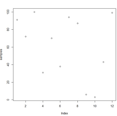

Matrices

Having defined the arrays, now the next step is that of the matrices. To define a matrix it is possible to start from an array like those seen above. Let’s take samples for example. Let’s assign it to a variable M that we will use for the matrix.

M <- samples
> M
 [1]  91  72 100  31  70  38  94  87   6   3  43  99

Now the next steps will be to convert an array to an array. The array is of 12 elements which can be converted for example into a 4×3 matrix. So to change the size of the array, you can directly define the dim() function.

dim(M) <- c(3,4)
> M
     [,1] [,2] [,3] [,4]
[1,]   91   31   94    3
[2,]   72   70   87   43
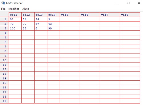
[3,]  100   38    6   99

As we can see, to convert an array to an array it is enough to vary its size. Another way to create or modify a matrix is through the fix () function which opens an editor that allows us to view the matrix and change its values.

A very common operation that is performed with matrices is transposition, this is possible through the simple t() function.

> t(M)
     [,1] [,2] [,3]
col1   91   72  100
col2   31   70   38
col3   94   87    6
col4    3   43   99

Lists

The objects seen so far had the characteristic of being able to contain only elements with values of the same type. Lists, on the other hand, allow you to group content of different types. To create a list, use the list() function with the elements inside it passed as parameters.

> t <- "word"
> a <- 5
> M <- sample(1:100, 12, replace=T)
> dim(M) <- c(3,4)
> mylist <- list(M,a,t)
> mylist
[[1]]
     [,1] [,2] [,3] [,4]
[1,]   91   35    6   33
[2,]   13   91   21   71
[3,]   67   27   31   30

[[2]]
[1] 5

[[3]]
[1] "word"

To access the elements of the list, simply indicate the name of the list with the index of the desired element. The indices start from the value 1.

> mylist[1]
[[1]]
     [,1] [,2] [,3] [,4]
[1,]   91   35    6   33
[2,]   13   91   21   71
[3,]   67   27   31   30

Dataframes

The most interesting type of data for working with data and using R as a tool for statistical and data processing and analysis is the dataframe. The dataframe is basically a data table with column headers and row indexes.

> a <- c(1,4,3,3,5)
> b <- c("BMW","Ford","Opel","Fiat","Alfa Romeo")
> c <- c(TRUE,TRUE,FALSE,FALSE,FALSE)
> df <- data.frame(a,b,c)
> df
  a          b     c
1 1        BMW  TRUE
2 4       Ford  TRUE
3 3       Opel FALSE
4 3       Fiat FALSE
5 5 Alfa Romeo FALSE

To access the elements of a dataframe column

> df$a
[1] 1 4 3 3 5

To access the elements of a row of the dataframe

> df[,2]
[1] "BMW"        "Ford"       "Opel"       "Fiat"       "Alfa Romeo"

Functions

The commands and functions present inside R are many, but they certainly cannot always cover the necessary. Moreover, often a series of instructions, commands and functions can be enclosed in a single operation, which we will define as a specific function.

For example, let’s create a function that calculates the area of the circle given the radius that we will call CircleArea. To define this function:

> CircleArea <- function(radius){
+     radius*radius*pi
+ }

Now that the function is defined we can call it whenever we need it in the following way.

> CircleArea(12)
[1] 452.3893