Forward kinematics

Post Views: 9,657

Forward kinematics allows us to determine the position and orientation of the end-effector in terms of the joint variables. A simple way to explain direct kinematics is to take a very simple case and apply the basic methodologies of this technique to it.

The manipulator with 2 links and 2 joints

A very simple case of robotics with which to apply direct kinematics is the 2-link and 2-joint manipulator. Now the classic problem of direct kinematics will be that, given the length of links l₁ and l₂, and the angles assumed by the two joints θ₁ and θ₂,, to derive the position of the effective end with the coordinates x and y.

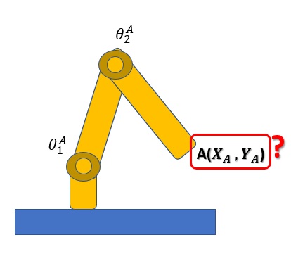
Forward Kinematics - il problema della cinematica diretta

In practical cases, manipulators often have internal sensors that allow to know in real time the position or angle of the various joints. Therefore we will take for granted the knowledge of the values of the two angles θ₁ and θ₂ which will be used as base values for our calculations.

The first thing to do will be to establish a fixed coordinate system, called the base frame. In the case of manipulators, the base of the manipulator (opposite end to the effective end) is referred to as the basis of the coordinates O₀x₀y₀.

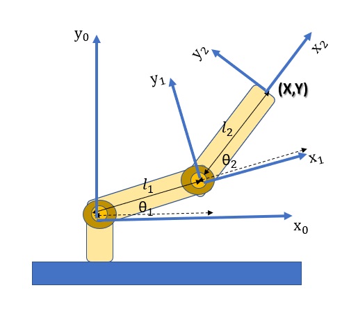
Forward Kinematics - base frame e sistemi di coordinate cartesiane

The (x, y) coordinates of the tool are expressed as:

$x = x_2 = l_1 cos \theta_1 + l_2 cos (\theta_1 + \theta_2)$

$y = y_2 = l_1 sin \theta_1 + l_2 sin (\theta_1 + \theta_2)$

Where l₁and l₂ are the lengths of the two links. The orientation of the tool frame relative to the base frame is also given by the direction of the cosines of the x₂ and y₂ axes with respect to the x₀ and y₀ axes.

$x_2 \cdot x_0 = cos(\theta_1 + \theta_2)$

$x_2 \cdot y_0 = -sin(\theta_1 + \theta_2)$

$y_2 \cdot x_0 = sin(\theta_1 + \theta_2)$

$y_2 \cdot y_0 = cos(\theta_1 + \theta_2)$

These four equations can be combined to obtain an orientation matrix.

$\begin{bmatrix} x_2 \cdot x_0 & y_2 \cdot x_0 \\ x_2 \cdot y_0 & y_2 \cdot y_0 \end{bmatrix} = \begin{bmatrix} cos(\theta_1 + \theta_2) & -sin(\theta_1 +\theta_2) \\ sin(\theta_1 + \theta_2) & cos(\theta_1 + \theta_2) \end{bmatrix}$

The equations we have just defined are called the forward kinematic equations and sno specific to the manipulator under consideration.

More complex cases – the Denavit-Hartenberg procedure

The case of the 2-link and 2-joint manipulator is a basic example, but other more advanced cases can lead to equations that are too complex and often not easily writable.

In any case, there is a general procedure that allows you to establish a coordinate system for each joint, and then to pass from one system to another through matrix transformations. This procedure is called the Denavit-Hartenberg procedure.

In this procedure, homogeneous coordinates and homogeneous transformations will be used to simplify the transformation between the different coordinate systems

There are therefore conventions, called Denavit-Hartenberg conventions.

The numbering of links and joints

The links are numbered from 0 to n starting from the base and arriving at the effective end, and are indicated with $L_0, L_1,…, L_n$ . This describes a serial manipulator with a chain of n + 1 links. This manipulator will consequently have n joints, which will be indicated in turn with $J_1,…, J_n$ .
The link $L_i$ will be the one that connects the joint $J_i$ with the one $J_ {i + 1}$ .

Assignment of the z axes of the different reference systems (frames)

Each link $L_i$ is associated with a frame of integral coordinates $S_i = (O_i, x_i, y_i, z_i)$ whose axis $z_i$ coincides with l ‘axis of the joint $J_ {i + 1}$ , ie of the joint downstream in the chain (the one closest to the effective end). Since the joints generally rotate on a plane, z is indicated as the axis perpendicular to this plane.

The basic element: link-joint

Therefore the Denavit-Hartenberg procedure mainly consists of considering as the basic element of a manipulator, a pair of joints with the link that joins them. Each base element thus defined will correspond to a coordinate transformation matrix

There are therefore two joints $J_i$ and $J_ {i + 1}$ and the link $L_i$ interposed, with the two reference systems defined together $S_ {i-1} = (O_ {i-1}, x_ {i-1}, y_ {i-1}, z_ {i-1})$ and $S_i = (O_i, x_i, y_i, z_i)$ .

In choosing the reference systems, proceed as follows:

the axis $z_ {i-1}$ is chosen coincident with the axis of the joint $J_ {i-1}$
the axis $z_i$ coinciding with the axis of the joint $J_i$ ;
the $x_ {i-1}$ axis can be freely chosen, but it is convenient to place it in the direction of the next joint, and it intersects with $z_ {i-1}$ in correspondence of the center of the joint $J_ {i-1}$ (chosen as origin);
the $x_i$ axis runs along the common normal between the $z_ {i-1}$ and $z_i$ axes;
the axes $y_ {n-1}$ and $y_n$ are chosen in order to complete the respective left-handed triples.

The transformation is then described by four Denavit-Hartenberg parameters:

$d$ which is the distance of the $z_ {i-1}$ axis from the common normal; in case there are infinite common normals (axes $z_i$ e and $z_ {i-1}$ parallel) the value of $d$ will be chosen more convenient;
$\ theta$ is the angle of rotation around the $z_ {i-1}$ axis needed to align $x_ {i-1}$ with [ latex] x_i [/latex];
$a$ (sometimes also referred to as $r$ is the minimum distance between the axes $z_ {i-1}$ and $z_i$ ;
$\alpha$ is the angle of rotation around the common normal (ie around $x_i$ ) to align the $z_ {i-1}$ axis to $z_i$ .

It can be seen that the $x_i$ axis is perpendicular to both the $z_ {i-1}$ axis and the $z_i$ axis and intersects both.

Coordinate transformation

Each arm-joint pair can be described as a coordinate transformation operation between the two reference systems associated with the joints.

If you choose to orient the $x_i$ axis along the common normal between the $z_ {i-1}$ and $z_i$ axes, the transformation matrix is defined as a series of two consecutive rototranslations:

${}^{i-1}T_i = Trans_{z_{i-1}} (d_i) \cdot Rot_{z_{i-1}} (\theta_i) \cdot Trans_{x_i}(r_i) \cdot Rot_{x_i} (\alpha_i)$

Where

$Trans_{z_{i-1}} (d_i) = \begin{pmatrix} 1 & 0 & 0 & 0 \\ 0 & 1 & 0 & 0 \\ 0 & 0 & 1 & d_n \\ 0 & 0 & 0 & 1 \end{pmatrix}$

$Rot_{z_{i-1}} (\theta_i) = \begin{pmatrix} \cos \theta_i & -\sin \theta_i & 0 & 0 \\ \sin \theta_i & \cos \theta_i & 0 & 0 \\ 0 & 0 & 1 & 0 \\ 0 & 0 & 0 & 1 \\ \end{pmatrix}$

$Trans_{x_i} (r_i) = \begin{pmatrix} 1 & 0 & 0 & r_i \\ 0 & 1 & 0 & 0 \\ 0 & 0 & 1 & 0 \\ 0 & 0 & 0 & 1 \\ \end{pmatrix}$

$Rot_{x_i} (\alpha_i) = \begin{pmatrix} 1 & 0 & 0 & 0 \\ 0 & \cos \alpha_i & -\sin \alpha_i & 0 \\ 0 & \sin \alpha_i & \cos \alpha_i & 0 \\ 0 & 0 & 0 & 1 \\ \end{pmatrix}$

From here we obtain the complete transformation matrix:

${}^{i-1}T_i = \begin{pmatrix} \cos \theta_i & -\sin \theta_i \cos \alpha_i & \sin \theta_i \sin \alpha_i & r_i \cos \theta_i \\ \sin \theta_i & \cos \theta_i \cos \alpha_i & -\cos \theta_i \sin \alpha_i & r_i \sin \theta_i \\ 0 & \sin \alpha_i & \cos \alpha_i & d_i \\ 0 & 0 & 0 & 1 \\ \end{pmatrix}$

Now that we know the coordinate transformation matrix for each single link-joint base element, it is possible to apply direct dynamics on any type of chain manipulator. It is sufficient to break down the manipulator, however complex, into its basic elements, calculate the transformation matrices for each element, and then multiply them to obtain a general matrix.

Let’s see some examples of more complex manipulators.

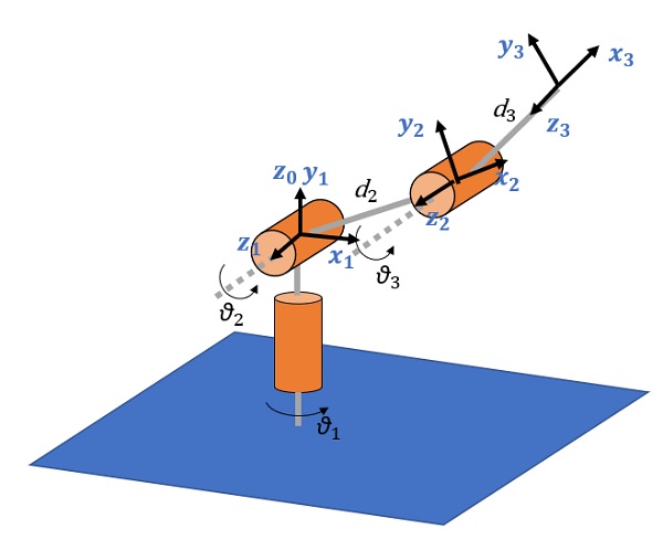
Three-arm planar manipulator

The three-arm manipulator is made up of three basic elements, whose joints all rotate on the same plane.

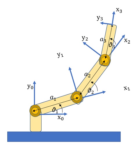
First, then, the four Denavit-Hartenberg parameters are defined for each base element and reported in a table.

BASE Element	$a_i$	$\alpha_i$	$d_i$	$\theta_i$
1	$a_1$	$0$	$0$	$\theta_1$
2	$a_2$	$0$	$0$	$\theta_2$
3	$a_3$	$0$	$0$	$\theta_3$

From the basic elements table it can be seen that the transformation matrices will be identical:

$T_i^{i-1} = \begin{bmatrix} cos \theta_i & -sin \theta_i & 0 & a_i cos \theta_i \\ sin \theta_i & cos \theta_i & 0 & a_i sin \theta_i \\ 0 & 0 & 1 & 0 \\ 0 & 0 & 0 & 1 \end{bmatrix} i = 1,2,3$

and therefore the general transformation will be:

$T_3^0 = T_1^0 T_2^1 T_3^2$

$T_3^0 = \begin{bmatrix} c_{123} & -s_{123} & 0 & a_1 c_1 + a_2 c_{12} + a_3 c_{123} \\ s_{123} & c_{123} & 0 & a_1 s_1 + a_2 s_{12} + a_3 s_{123} \\ 0 & 0 & 1 & 0 \\ 0 & 0 & 0 & 1 \end{bmatrix}$

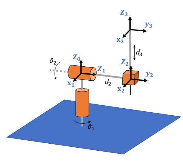
Spherical manipulator

Also for the spherical manipulator it is possible to create a table with the four Denavit-Hartenberg parameters for each base element. Here too we have 3 basic elements, but this time the transformation matrices will be different for each basic element.

BASE Element	$a_i$	$\alpha_i$	$d_i$	$\theta_i$
1	$0$	$-\pi/2$	$0$	$\theta_1$
2	$0$	$\pi/2$	$d_2$	$\theta_2$
3	$0$	$0$	$d_3$	$0$

The three transformation matrices of the coordinates corresponding to the single elements will therefore be the following:

$T_1^0 = \begin{bmatrix} c_1 & 0 & -s_1 & 0 \\ s_1 & 0 & c_1 & 0 \\ 0 & -1 & 0 & 0 \\ 0 & 0 & 0 & 1 \end{bmatrix}$

$T_2^1 = \begin{bmatrix} c_2 & 0 & s_2 & 0 \\ s_2 & 0 & -c_2 & 0 \\ 0 & 1 & 0 & d_2 \\ 0 & 0 & 0 & 1 \end{bmatrix}$

$T_3^2 = \begin{bmatrix} 1 & 0 & 0 & 0 \\ 0 & 1 & 0 & 0 \\ 0 & 0 & 1 & d_3 \\ 0 & 0 & 0 & 1 \end{bmatrix}$

And so the general transformation matrix will be:

$T_3^0 = T_1^0 T_2^1 T_3^2$

$T_3^0 = \begin{bmatrix} c_1 c_2 & -s_1 & c_1 s_2 & c_1 s_2 d_3 - s_1 d_2 \\ s_1 c_2 & c_1 & s_1 s_2 & s_1 s_2 d_3 + c_1 d_2 \\ -s_2 & 0 & c_2 & c_2 d_3 \\ 0 & 0 & 0 & 1 \end{bmatrix}$

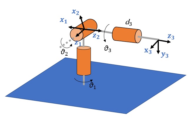
Anthropomorphic manipulator

Even for complex manipulators like the anthropomorphic one, the approach remains almost the same. Here, too, three basic elements are defined and the following table with the corresponding Denavit-Hartenberg properties.

BASE Element	$a_i$	$\alpha_i$	$d_i$	$\theta_i$
1	$0$	$-\pi/2$	$0$	$\theta_1$
2	$a_2$	$0$	$0$	$\theta_2$
3	$a_3$	$0$	$0$	$\theta_3$

The three coordinate transformation matrices are obtained from the table (two are equal).

$T_1^0 = \begin{bmatrix} c_1 & 0 & s_1 & 0 \\ s_1 & 0 & -c_1 & 0 \\ 0 & 1 & 0 & 0 \\ 0 & 0 & 0 & 1 \end{bmatrix}$

$T_i^{i-1} = \begin{bmatrix} c_i & -s_i & 0 & a_i c_i \\ s_i & c_i & 0 & a_i s_i \\ 0 & 0 & 1 & 0 \\ 0 & 0 & 0 & 1 \end{bmatrix} i = 2,3$

From the three transformation matrices of the basic elements we obtain the general one:

$T_3^0 = T_1^0 T_2^1 T_3^2$

$T_3^0 = \begin{bmatrix} c_1 c_{23} & -c_1 s_{23} & s_1 & c_1 ( a_2 c_2 - a_3 c_{23}) \\ s_1 c_{23} & -s_1 s_{23} & -c1 & s_1 ( a_2 c_2 + a_3 c_{23} \\ s_{23} & c_{23} & 0 & a_2 s_2 + a_3 s_{23} \\ 0 & 0 & 0 & 1 \end{bmatrix}$

Spherical wrist

Another popular manipulator is the spherical wrist, often connected as an effective end to other manipulators.

BASE Element	$a_i$	$\alpha_i$	$d_i$	$\theta_i$
1	$0$	$-\pi/2$	$0$	$\theta_1$
2	$0$	$\pi/2$	$0$	$\theta_2$
3	$0$	$0$	$d_3/latex]</td><td>[latex]\theta_3$

The three coordinate transformation matrices are obtained from the table (two are equal).

$T_1^0 = \begin{bmatrix} c_1 & 0 & -s_1 & 0 \\ s_1 & 0 & c_1 & 0 \\ 0 & -1 & 0 & 0 \\ 0 & 0 & 0 & 1 \end{bmatrix}$

$T_2^1 = \begin{bmatrix} c_2 & 0 & s_2 & 0 \\ s_2 & 0 & -c_2 & 0 \\ 0 & 1 & 0 & 0 \\ 0 & 0 & 0 & 1 \end{bmatrix}$

$T_3^2 = \begin{bmatrix} c_3 & 0 & -s_3 & 0 \\ s_3 & 0 & c_3 & 0 \\ 0 & 0 & -1 & d_3 \\ 0 & 0 & 0 & 1 \end{bmatrix}$

From the three transformation matrices of the basic elements we obtain the general one:

$T_3^0 = T_1^0 T_2^1 T_3^2$

$T_3^0 = \begin{bmatrix} c_1 c_2 c_ - s_1 s_3 & -c_1 c_2 s_3 - s_1 c_3 & c_1 s_2 & c_2 s_2 d_3 \\ s_1 c_2 c_3 + c_1 s_3 & -s_1 c_2 s_3 + c_1 c_3 & s_1 s_2 & s_1 s_2 d_3 \\ - s_2 c_3 & s_2 s_3 & c_2 & c_2 d_3 \\ 0 & 0 & 0 & 1 \end{bmatrix}$