Robot Dynamics

Post Views: 10,788

The dynamics in robotics, in English defined as robot dynamics, studies the forces acting on a robotic mechanism and the accelerations that these forces produce. The robotic mechanism is generally considered as a rigid system, in order to apply the dynamic laws of rigid bodies.

Robot Dynamics - La dinamica in robotica

Introduction to Robot dynamics

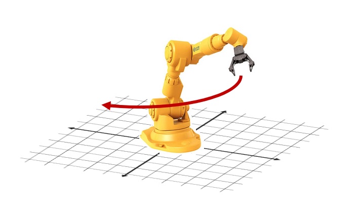
When dealing with a robotic mechanism, such as a manipulator robot, one must take into account its basic functionality: its correct positioning. When this has to move from a starting position to a target position, we will need to know all the dynamic properties of the manipulator, in order to predict how the various forces and accelerations will affect the movement.

If, for example, too small forces are applied to produce the movement, we may have too slow a movement, while if they are too strong, we risk making the manipulator collide with other objects in the environment, swinging excessively with respect to the desired position.

It is for this reason that dynamic equations of motion have been defined in robotics. But their derivation is certainly not a very simple operation to do. In particular, the complexity increases with the increase in the number of degrees of freedom of the robotic system, and the many non-linearities present in such systems.

For this purpose, techniques based on Lagrangian dynamics come to our aid. These techniques allow us to systematically derive the equations of motion of robotic systems.

The two main problems in robotic dynamics are:

Forward dynamics: given the forces, the accelerations are obtained
Inverse dynamics: given the accelerations the forces are obtained

Forward dynamics or simply dynamics. It is mainly used for simulation.

Inverse dynamics is instead used for direct control over the motion and forces involved in a robotic mechanism, or even for the study of the trajectory, for optimization, for the design of robotic mechanisms.

Other problems concerning robot dynamics are:

Calculation of coefficients in the equation of motion
Identification of inertial parameters
Hybrid dynamics: given some forces and some accelerations, the missing forces and accelerations are obtained.

Equations of motion

The equations of motion for a physical system describe its motion as a function of time and optional control inputs. In the general form, the equations of motion take the following generalized form.

$F (q(t), \dot{q}(t), \ddot{q}(t), u(t), t) = 0$

where

t is the variable time
q is the vector of generalized coordinates, for example the vector of the angles of the joints of a manipulator
$\dot{q}$ is the velocity vector (first derivative of q)
$\ddot{q}$ is the vector of accelerations (second deviation of q)
u is the vector of the input control parameters

The equations of motion allow to obtain a mapping between the control space and the commands sent to the actuators, and between the state space and the robot movement.

In robotics some assumptions are introduced:

Rigid bodies: in robotics, all systems, such as manipulators for example, are considered to be made up of a set of rigid parts (links) connected to each other by joints regulated by a motor (actuated joints). This assumption allows us to use the theory of rigid body dynamics.
D’Alembert’s principle: internal forces (constraint forces) are conservative. These forces act on each joint to prevent any movement outside the joint axes.

The equations of motion for Manipulators

Manipulators are a particular case of articulated systems where at least one of the links is fixed to the environment. The equations of motion for a manipulator can be written as follows:

$M(q) \ddot{q} + \dot{q}^T C(q) \dot{q} = \tau + \tau_g (q)$

where the robot degrees of freedom can be written:

$n=dim(q)$

and where

M(q) is the n×n inertial matrix,
C(q) is the n×n×n Coriolis tensor,
$\tau$ is the n-dimensional vector of the torsions of the actuated joints
$\tau_g(q)$ is the n-dimensional vector of the torsions of external joints caused by gravity

Robot dynamics - angoli del robot manipolatore

Contrary to the general form $F (q (t), \ dot {q} (t), \ ddot {q} (t), u (t), t) = 0$ , this expression is invariant over time, in fact t does not appear in the formula. In this way, knowing the current state $(q, \ dot {q})$ and the torque applied to the joint $\ tau$ , one can directly calculate the resulting accelerations at the joints $\ ddot {q}$ . This operation is known as forward dynamics.

The system therefore has no memory. Regardless of how a particular state has been reached, starting from that state there will always be an equal acceleration.

The inertia matrix M and the Coriolis tensor

The inertia matrix M and the Coriolis tensor can be derived from the inertia of the links and their Jacobian:

$M(q) = \sum_i J_i^t(q)^T m_i J_i^t (q) + J_i^R(q)^T I_i J_i^R(q)$

$\dot{q}^T C(q) = \sum_i J_i^t(q)^T m_i \dot{J}_i^t (q) + J_i^R(q)^T I_i \dot{J}_i^R(q) - J_i^R (q)^T( I_i J_i^R \dot{q}) \times J_i^R$

where mi is the total mass of link i, Ii is its inertia matrix, and Ji is the Jacobian of the frame attached to link i.

The rotational Jacobian $J_i ^ R$ is such that the angular velocity ωi of the frame of the link with respect to the inertial frame satisfies $\ omega_i = J_i ^ R \ dot {q}$
the translational Jacobian $J_t ^ C$ is such that the linear velocity $\ dot {p} _i$ of the origin of the inertial link frame satisfies $\ dot {p} _i = J_i ^ t \ dot {q}$ .

Torsion of gravity and external forces

The external forces applied to the system can be expressed through a similar formula:

$\tau_{ext} (q) = \sum_i J_i^t (q)^T f_{ext,i} + J_i^R (q)^T \tau_{ext,i}$

where $f_{ext, i}$ denotes the resultant of the external forces applied to link i of the robot and $\tau_{ext,i}$ is the moment of these forces. Together they form the foreign key applied to the link. The coordinates of the wrench should be consistent with the definition of our Jacobian matrices. Assuming that the image of our Jacobian matrices are expressed in the inertial frame, then the coordinates of the wrench should be expressed in the initial frame in the same way.

We consider gravity as our external force. Assuming that the frame attached to link i is located in the center of the mass of the link, the torsions of the joint caused by gravity can be expressed:

$\tau_g(q) = \sum_i m_i J_i^t (q)^T g$

By definition, the Jacobian Jcom of the center of mass is such that

$\sum_i m_i J_{com} = \sum_i m_i J_i^t$

and therefore the previous expression can be changed to:

$\tau_g (q) = m J_{com} (q) g$

Dynamic models

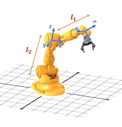
The equations of motion depend on the dynamic model corresponding to the robotic mechanism under study. The dynamic model is nothing more than a description of the robotic mechanism in terms of the parts that compose it: links, joints and the parameters that characterize these components.

In particular, a dynamic model consists of:

a kinematic model of the robotic mechanism
a set of inertial parameters

10 inertial parameters are required to define the inertia of a single rigid body (mass, position of the center of mass, and 6 inertial parameters of rotation). Therefore each dynamic model will have 10 inertial parameters for each component (identifiable rigid body) of the robotic mechanism.

However, when the bodies are connected together to form a robotic mechanism, such as a manipulator, some degrees of freedom of the system are eliminated. In fact some of them will no longer have an effect on the dynamic behavior of the system.

The basic procedure, once a kinematic model has been identified and a series of measurements of its dynamic behavior have been carried out, will therefore be to identify the values of a set of basic inertial parameters which are then those observable experimentally.

There are several methodologies on which, given a robotic mechanism, a dynamic model can be derived. However the best known are:

Lagrangian method
Newton-Euler method

The Lagrangian method is simpler and more systematic, while the second is more efficient especially from the point of view of computational calculation.

Lagrangian method

The Lagrange method is based on the calculation of a certain value, called the Lagrangian, which belongs to the mechanical system from which the model is derived. Lagrange’s is an energetic approach that allows to derive the equations of dynamics in symbolic (or closed form), that is, non-numerical form, thus facilitating the study of the properties and the analysis of control schemes.

The Lagrangian is equal to the difference between the kinetic energy T and the potential energy U of the system:

$L = T – U$

This particular value depends both on dynamic parameters (masses and moments of inertia of the links) and on geometric parameters (length of the links).

It can be shown that the following Lagrange equations exist

$\frac {d} {dt} \frac {\partial L} {\partial \dot{q}_i} - \frac {\partial L} {\partial q_i} = \xi_i , i = 1, ... , n$

Where with $\ xi_i$ we indicate the generalized forces associated with the generalized coordinates $q_i$ .

The peculiarity of this method is that the Lagrangian magnitude is expressed in symbolic form and can be manipulated and elaborated through a systematic approach. Once the expression of the Lagrangian has been obtained, the corresponding dynamic model can be derived, thanks to a series of equations, called Euler-Lagrange equations, which can be directly deduced from it.

For example, for a robotic manipulator the kinetic energy is given by:

$T(q, \dot{q}) = \frac{1}{2} \dot{q}^T B(q)\dot{q}$

Where B is the Inertia matrix. While the potential energy is given by:

$U(q) = \sum_{i=1}^{n} - m_i g^T p_{C_i}$

From which the Lagrangian equation is obtained:

$L(q, \dot{q} ) = T(q, \dot{q}) - U(q) = \frac{1}{2} \sum_{i=1}^{n} \sum_{j=1}^{n} b_{ij} (q) \dot{q}_i \dot{q}_j + \sum_{i=1}^{n} m_i q^T p_{C_i}$

By deriving and adding the appropriate operations, we arrive at the matrix form:

$B(q) \ddot{q} + C (q, \dot{q}) \dot{q} + g(q) = \tau$

$B(q) \ddot{q}$ Inertial terms
$C (q, \dot{q}) \dot{q}$ Centrifugal and Coriolis terms
$g(q)$ Gravitational terms
$\tau$ Couples at the joints

Where $\dot {q}$ and $\ddot {q}$ are the joint velocities and accelerations, $B (q)$ is the inertial matrix of the manipulator, $C (q, \dot{q}) \dot{q}$ is a velocity term describing centrifugal and Coriolis effects, while $g (q)$ is a gravitational term dependent only on the configuration. Finally $\tau$ describes the effect of any forces and moments exerted by the external environment on the robot.

The dynamic model of the manipulator, as shown in the previous equation, was formulated in the joint space. Nevertheless it is possible to obtain a formulation also in the operative space.

Finally, it is important to note that in the derivation of the dynamic model, the actuation system, consisting of engines and transmission system, was not taken into account. The actuation system contributes to the dynamic effects in various ways: for example by changing the parameters of inertia and masses of the links, and by introducing their own dynamics (electromechanical) and possible non-linear effects such as play, friction and elasticity. All these effects can however be considered by introducing appropriate modifications to the dynamic model. Viscous friction pairs and static friction pairs can also act on the manipulator.

There are systematic methods to derive the coefficients of the inertia matrix and
then, by derivation, the centrifugal and Coriolis ones. However, the writing of the dynamic model based on Lagrange’s equations, while giving rise to a model in closed form, easily interpretable and usable in the synthesis of the controller, constitutes an inefficient procedure from a computational point of view.

Newton-Euler method

An alternative way to formulate the dynamic model is that which goes by the name of the Newton-Euler method.

This method is based on the use of two equations: Newton’s dynamic equation, according to which the sum of the forces acting on a mechanical system is equal to the variation of the momentum, and the Euler’s dynamic equation, according to which the sum of moments is equal to the variation of the moment of the momentum.

The Newton-Euler method therefore consists in writing the balance of forces (Newton’s equations) and of moments (Euler’s equations) acting on each link, highlighting the interactions with the contiguous links in the kinematic chain. In this way, a system of equations is obtained that can be solved recursively, by propagating the speeds and accelerations from the base towards the end organ, and the forces and moments in the opposite direction.

A system of equations is obtained that can be solved recursively, by propagating the velocities and accelerations from the base towards the end organ, and the forces and moments in the opposite direction. Recursion makes the Newton-Euler algorithm computationally efficient.

These recursive formulas can be evaluated both symbolically and numerically, however it is only in the second mode, the numerical one, that recursion makes the Newton-Euler algorithm particularly efficient from a computational point of view.

Lagrange vs. Newton-Euler

Although the Lagrangian and Newton-Euler approaches, solved in symbolic form, ultimately produce the same mathematical model for the dynamics of a manipulator, it is possible to highlight some differences between these two formulations.

Lagrange’s formulation:

it is systematic and easily understood
it provides the equations of motion in a compact analytical form, highlighting the inertia matrix, the centrifugal and Coriolis terms, and the gravitational terms. These elements are useful for designing a model-based controller.
it lends itself to the introduction of more complex dynamic effects into the model (deformability at joints or in links)

Newton-Euler formulation:

it is a recursive, computationally efficient method
it is recommended for use in real time

Algorithms in Robot dynamics

From a practical point of view, currently 3 different algorithms are mainly used in robot dynamics:

Recursive Newton-Euler algorithm (RNEA). This algorithm solves the inverse dynamics problems, and has a computational complexity of O (n). It can be used to calculate C in the equation of motion.
Articulated-body algorithm (ABA). This algorithm solves the problems of forward dynamics, and has a computational complexity of O (n).
Composite-rigid-body algorithm (CRBA). This algorithm computes the inertial matrix of the joint space, M, and has a computational complexity of O (n2).

Further information on the functionality of these algorithms and their specifications will be discussed in other articles.

References

Robot Dynamics from Scholarpedia
Equations of motion from Scaron.info