The Random Forest algorithm in Machine Learning with Python

Random Forest is a machine learning algorithm that is based on building a set of decision trees. Each tree is built using a random subset of the training data and produces a prediction. Finally, the predictions from all the trees are combined through majority voting to get the final prediction.

[wpda_org_chart tree_id=22 theme_id=50]

The Random Forest algorithm

The Random Forest algorithm is a machine learning technique that belongs to the category of ensemble methods, i.e. methods that combine several weaker models to create a stronger and more robust model. The idea behind Random Forest is to create an ensemble of decision trees, each built on a different subset of the data and with some degree of randomness in their training. The predictions of each tree are combined by majority vote (in the case of classification) or by averaging (in the case of regression) to obtain the final prediction.

Here’s how the Random Forest algorithm works:

• Bagging (Bootstrap Aggregating): The Random Forest ensemble begins by creating several subsets of the training data. These subsets are created using replacement sampling from the original data. This process is known as bagging. Each subset represents a unique training set for a single tree.
• Tree Creation: For each subset of data, a decision tree is created. Each tree is trained using only a subset of the data, but may have differences in structures and node splits due to random sampling.
• Majority Vote: Once all trees have been trained, predictions from each tree are combined. In the case of classification, the class predicted by the majority of trees (majority vote) is taken into consideration. In the case of regression, the predictions of all trees are averaged.
• Reducing Overfitting: The use of different subsets of data and the randomness introduced during tree building help reduce overfitting, which is a common issue in single decision trees.

Random Forest has several benefits, including:

• Improve generalization on new data by reducing overfitting.
• It is resistant to noise and atypical values in the data.
• It does not require special data preparation.
• It can handle both categorical and numerical data.

A bit of history

The Random Forest algorithm was introduced by Leo Breiman in 2001. Breiman was an influential statistician and professor at the University of California, Berkeley. Leo Breiman’s original article, titled “Random Forests,” was published in the journal “Machine Learning” in 2001. The article presented the idea of creating an ensemble of decision trees with the goal of improving the performance of prediction and robustness compared to individual trees.

The main motivation behind building Random Forest was to address the limitations and weaknesses of single decision trees. Decision trees can be prone to overfitting, especially when they are deep and complex, and can be sensitive to small changes in the data. Breiman’s goal was to develop an approach that could improve generalization, reduce overfitting, and make the machine learning process more robust.

The key to Random Forest’s effectiveness lies in the idea of building different decision trees on random subsets of the data and combining their predictions. This forecast aggregation process reduces variance and improves the stability of the overall forecasts.

Since its introduction, Random Forest has become one of the most popular and widely used machine learning models. It is suitable for a wide range of classification and regression problems and has been shown to perform well in many applications. Its flexibility, robustness, and ability to handle heterogeneous data have made it a vital tool for many data scientists and machine learning researchers.

Suggested Book

If you are interested in Machine Learning with Python I suggest you read this book:

Machine Learning with Python Cookbook

Random Forest with the scikit-learn library

In Python, you can use the scikit-learn library to implement the Random Forest algorithm and build models based on Random Forest. This algorithm can be used for two different Machine Learning approaches.

• Classification
• Regression

Classification with Random Forest

Classification Random Forest is a variant of the Random Forest algorithm used to solve classification problems. The goal of Classification Random Forest is to predict which class an input instance belongs to.

Here’s how you can use Classification Random Forest with the scikit-learn library in Python:

1. Import libraries:

from sklearn.datasets import load_iris
from sklearn.model_selection import train_test_split
from sklearn.ensemble import RandomForestClassifier
from sklearn.metrics import accuracy_score

2. Load the dataset and split the data:

#Upload the Iris dataset as an example
iris = load_iris()
X = iris.data
y = iris.target

#Divide the dataset into training and test sets<code>
X_train, X_test, y_train, y_test = train_test_split(X, y, test_size=0.2, random_state=42)

3. Create and train the Random Forest classifier:

# Create the Random Forest classifier with 100 trees
clf = RandomForestClassifier(n_estimators=100, random_state=42)

#Train the classifier on the training set
clf.fit(X_train, y_train)

4. Make predictions and calculate accuracy:

# Make predictions on the test set
predictions = clf.predict(X_test)

# Calculate the accuracy of forecasts
accuracy = accuracy_score(y_test, predictions)
print("Accuracy:", accuracy)

In this example, we are using the Iris dataset to create a Random Forest classifier. After dividing the dataset into training and test sets, we create a RandomForestClassifier object with 100 trees (n_estimators=100). We then train the classifier on the training data and make predictions on the test set. The accuracy of the predictions is calculated using the accuracy_score function. By running it you get the accuracy value.

Accuracy: 1.0

For further description of the validity of the newly trained model, we can add additional useful graphical representations, as well as the confusion matrix.

import matplotlib.pyplot as plt
import numpy as np
from sklearn.metrics import confusion_matrix
import seaborn as sns
# View the importance of features
feature_importances = clf.feature_importances_
feature_names = iris.feature_names

plt.barh(range(len(feature_importances)), feature_importances, align='center')
plt.yticks(np.arange(len(feature_names)), feature_names)
plt.xlabel('Importance of Features')
plt.title('Importance of Features in Random Forest')
plt.show()

# View the confusion matrix
cm = confusion_matrix(y_test, predictions)
plt.figure(figsize=(8, 6))
sns.heatmap(cm, annot=True, fmt='g', cmap='Blues', xticklabels=iris.target_names, yticklabels=iris.target_names)
plt.xlabel('Predictions')
plt.ylabel('Real values')
plt.title('Random Forest Confusion Matrix')
plt.show()

By also executing this part of code we will obtain the following two views. First, a diagram representing the importance of features to the validity of the model’s predictions: a horizontal bar graph showing the relative importance of each feature in the Random Forest model. This can give you an idea of which features are most influential in the model’s decision-making process.

And then the confusion matrix of the prediction results obtained from our model. A confusion matrix is a visual representation of the model’s performance. Shows how many samples were classified correctly and how many incorrectly for each class. In this case, the classes correspond to the types of irises in the dataset.

Remember that it’s important to adjust the algorithm’s hyperparameters, such as number of trees, maximum tree depth, and maximum number of attributes to consider for splitting (max_features), to get the best results on your specific classification challenge.

If you want to delve deeper into the topic and discover more about the world of Data Science with Python, I recommend you read my book:

Python Data Analytics 3rd Ed

Fabio Nelli

Regression with Random Forest

Regression Random Forest is a variant of the Random Forest algorithm that is used for regression rather than classification problems. While the standard Random Forest algorithm is often used for classification problems where the goal is to predict a class or category, Random Forest Regression is used to predict continuous numeric values.

Regression Random Forest works similar to the classification version, but with some differences in the output and the process of aggregating the predictions:

1. Tree building: As in the Random Forest for classification, different decision trees are built using random subsets of the training data. Each tree is trained to predict a numeric value rather than a class.
2. Tree predictions: After trees are created, each tree makes predictions on test data. In this case, the predictions will be numerical values.
3. Forecast Aggregation: The forecasts from each tree are combined to get the final forecast. Instead of using majority voting as in classification, the average of the predictions of all trees is used. Thus, the final prediction is the average of the individual tree predictions.

The goal of the Regression Random Forest is to predict a continuous numeric value that represents an output characteristic of the problem. For example, it could be used to predict the price of a house based on its features, the amount of sales based on marketing variables, or any other problem where the output variable is a numeric value.

In Python, you can use the same scikit-learn library to implement Random Forest Regression using the RandomForestRegressor class.

Here’s how you can use Regression Random Forest with the scikit-learn library in Python:

1. Import libraries:

from sklearn.datasets import fetch_california_housing
from sklearn.model_selection import train_test_split
from sklearn.ensemble import RandomForestRegressor
from sklearn.metrics import mean_squared_error

2. Load the dataset and split the data:

# Upload the Californa Housing dataset as an examples
housing = fetch_california_housing()
X = housing.data
y = housing.target

# Divide the dataset into training and test sets
X_train, X_test, y_train, y_test = train_test_split(X, y, test_size=0.2, random_state=42)

3. Create and train the Random Forest regressor:

# Create the Random Forest regressor with 100 trees
reg = RandomForestRegressor(n_estimators=100, random_state=42)

# Train the regressor on the training set
reg.fit(X_train, y_train)

4. Make predictions and calculate the root mean square error:

# Make predictions on the test set
predictions = reg.predict(X_test)

# Calculate the root mean squared error of the predictions<code>
mse = mean_squared_error(y_test, predictions)
print("Mean Squared Error:", mse)

In this example, we are using the Boston House Prices dataset to create a Random Forest regressor. After dividing the dataset into training and test sets, we create a RandomForestRegressor object with 100 trees (n_estimators=100). We then train the regressor on the training data and make predictions on the test set. The mean squared error (MSE) of the predictions is calculated using the mean_squared_error function. Running the code you will get the value of the MSE.

Mean Squared Error: 0.2553684927247781

Also in this case it is possible to add visualizations that can help us better understand the validity or otherwise of the Random Forest regression model.

import matplotlib.pyplot as plt
import seaborn as sns
import numpy as np

# Scatter plot between actual and predicted values
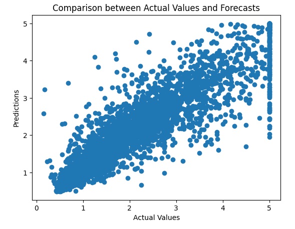
plt.scatter(y_test, predictions)
plt.xlabel('Actual Values')
plt.ylabel('Predictions')
plt.title('Comparison between Actual Values and Forecasts')
plt.show()

# View the importance of features
feature_importances = reg.feature_importances_
feature_names = housing.feature_names

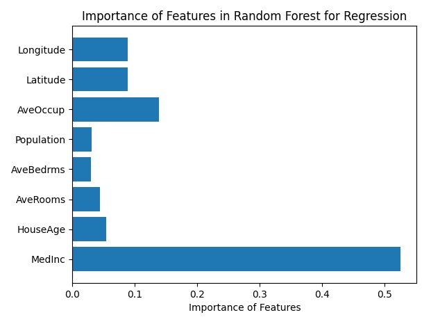
plt.barh(range(len(feature_importances)), feature_importances, align='center')
plt.yticks(np.arange(len(feature_names)), feature_names)
plt.xlabel('Importance of Features')
plt.title('Importance of Features in Random Forest for Regression')
plt.show()

# View the error distribution
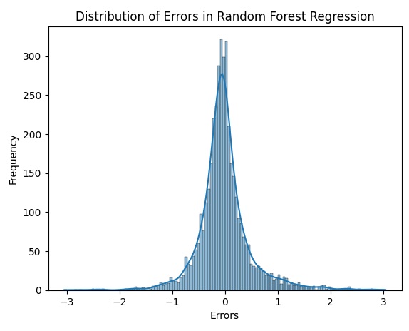
errors = y_test - predictions
sns.histplot(errors, kde=True)
plt.xlabel('Errors')
plt.ylabel('Frequency')
plt.title('Distribution of Errors in Random Forest Regression')
plt.show()

Running the code gives you three different views. The first visualization is a Scatterplot. A scatterplot showing the relationship between actual values and model predictions. Ideally, the dots should align with the diagonal line, indicating a good forecast.

Feature Importance: A horizontal bar graph showing the relative importance of each feature in the Random Forest model for regression.

Error Distribution: A histogram showing the distribution of errors, helping you understand the accuracy of the model across different predictions.

As always, it’s important to adjust the algorithm’s hyperparameters to get the best results on your specific regression challenge. You can explore various values for hyperparameters such as the number of trees, the maximum depth of trees, and the maximum number of attributes to consider for splitting (max_features).

Suggested book:

Machine Learning with PyTorch and Scikit-Learn

Some datasets for practicing classification problems with scikit-learn

If you want to get some Machine Learning practice working with classification problems, there are ready-made datasets to practice on. Here are some datasets you can use for practical examples with Classification Random Forest using scikit-learn without using the Iris dataset:

1. Breast Cancer Wisconsin (Diagnostic) Dataset: This dataset contains features extracted from images of fine aspirates of breast lumps and the goal is to classify whether a tumor is benign or malignant.
   • Upload the dataset: from sklearn.datasets import load_breast_cancer
2. Wine Dataset: This dataset contains chemical measurements of wines from three different varietals. The goal is to classify the variety of wine.
   • Upload the dataset: from sklearn.datasets import load_wine
3. Digits Dataset: This dataset contains images of handwritten digits and the goal is to classify which digit is represented.
   • Upload the dataset: from sklearn.datasets import load_digits
4. Heart Disease UCI Dataset: This dataset contains clinical information for patients and the goal is to classify whether or not a patient has heart disease.
   • Upload the dataset: UCI Machine Learning Repository
5. Bank Marketing Dataset: This dataset contains information on bank marketing campaigns and the objective is to classify whether or not a customer will subscribe to a term deposit.
   • Upload the dataset: UCI Machine Learning Repository
6. Titanic Dataset: This dataset contains information about the passengers of the Titanic and the goal is to classify whether or not a passenger will survive.
   • Upload the dataset: Kaggle

To use one of these datasets, you can import the appropriate dataset using the load_* function provided by sklearn.datasets. Be sure to read the documentation associated with the dataset to understand the characteristics, the output variable, and how to prepare the data for Random Forest model training.

Some datasets for practicing regression problems with scikit-learn

Here are some datasets you can use for practical examples with Regression Random Forest using scikit-learn:

1. California Housing Dataset: This dataset contains data on homes in the California area and the goal is to predict median home value.
   • Load dataset: from sklearn.datasets import fetch_california_housing
2. Diabetes Dataset: This dataset contains medical measurements related to diabetes and the goal is to predict disease progression one year later.
   • Load dataset: from sklearn.datasets import load_diabetes
3. Energy Efficiency Dataset: This dataset contains information on the energy performance of buildings and the objective is to predict energy efficiency.
   • Load dataset: UCI Machine Learning Repository
4. Concrete Compressive Strength Dataset: This dataset contains data on the compressive strength of concrete and the goal is to predict the compressive strength.
   • Load dataset: UCI Machine Learning Repository
5. Combined Cycle Power Plant Dataset: This dataset contains data on energy production in a power plant and the goal is to predict energy efficiency.
   • Load dataset: UCI Machine Learning Repository

To use one of these datasets, you can import the appropriate dataset using the load_* function provided by sklearn.datasets. Be sure to read the documentation associated with the dataset to understand the characteristics, the output variable, and how to prepare the data for training the Random Forest Regression model.