Questo è il quarto di una serie di articoli che illustrano come sviluppare un dendrogramma, utilizzando la libreria JavaScript D3, costruito in base ad una particolare struttura dati contenuta all’interno di un file JSON.
Leggi l’articolo:
- Come realizzare un dendrogramma con la libreria D3 (parte 1)
- Come realizzare un dendrogramma con la libreria D3 (parte 2)
- Come realizzare un dendrogramma con la libreria D3 (parte 3)
Nell’articolo precedente abbiamo realizzato un dendrogramma in cui si teneva conto delle distanze ultrametriche.
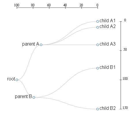
In questo articolo vedremo come sia possibile gestire una ulteriore distanza tra i vari nodi, distanza che verrà espressa all’interno del dendrogramma attraverso la posizione verticale dei vari nodi.
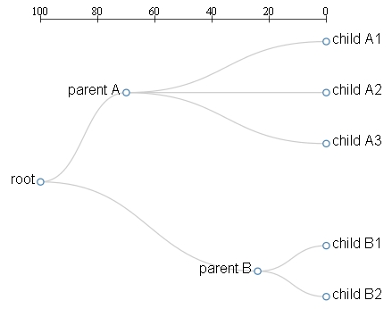
Abbiamo visto nei precedenti articoli che la posizione dei vari nodi del dendrogramma è esprimibile nella struttura JSON attraverso l’attribuzione dei valori (x,y) ai corrispettivi attributi x e y di ciascun nodo.
Quindi per ottenere il dendrogramma espresso in figura 2 editiamo la seguente struttura JSON, salvandola come dendrogram03.json.
{   "name": "root",
    "y" : 0,
    "x" : 100,
    "children": [
        {"name": "parent A",
         "y" : 30,
         "x" : 40,
         "children": [
             {"name": "child A1",
              "y" : 100,
              "x" : 0},
             {"name": "child A2",
              "y" : 100,
              "x" : 10},
             {"name": "child A3",
              "y" : 100,
              "x" : 40}     ]
          },{"name": "parent B",
          "y" : 21,
          "x" : 130,
          "children": [
              {"name": "child B1",
               "y" : 100,
               "x" : 80},
              {"name": "child B2",
               "y" : 100,
               "x" : 150}
           ]   }
] }
Come possiamo ben vedere, questa volta tutti i nodi hanno un valore x e un valore y definito al suo interno.
Adesso implementiamo la pagina Web con cui rappresenteremo il nostro dendrogramma.
<!doctype html>
<html>
<meta charset="utf-8">
<style>
.node circle {
     fill: #fff;
     stroke: steelblue;
     stroke-width: 1.5px;
}
.node {
     font: 20px sans-serif;
}
link {
     fill: none;
     stroke: #ccc;
     stroke-width: 1.5px;
}
line {
     stroke: black;
}
</style>
<script type="text/javascript" src="http://d3js.org/d3.v3.min.js">
var width = 600;
var height = 500;
var cluster = d3.layout.cluster()
     .size([height, width-200]);
var diagonal = d3.svg.diagonal()
     .projection (function(d) { return [x(d.y), y(d.x)];});
var svg = d3.select("body").append("svg")
     .attr("width",width)
     .attr("height",height)
     .append("g")
     .attr("transform","translate(100,0)");
xs = [];
ys = [];
function getXYfromJSONTree(node){
     xs.push(node.x);
     ys.push(node.y);
     if(typeof node.children != 'undefined'){
          for ( j in node.children){
                getXYfromJSONTree(node.children[j]);
          }
     }
}
var ymax = Number.MIN_VALUE;
var ymin = Number.MAX_VALUE;
var xmax = Number.MIN_VALUE;
var xmin = Number.MAX_VALUE;
d3.json("dendrogram03.json", function(error, json){
    getXYfromJSONTree(json);
    var nodes = cluster.nodes(json);
    var links = cluster.links(nodes);
    nodes.forEach( function(d,i){
         if(typeof xs[i] != 'undefined'){
              d.x = xs[i];
         }
         if(typeof ys[i] != 'undefined'){
              d.y = ys[i];
         }
    });

nodes.forEach( function(d){
    if(d.y > ymax)
        ymax = d.y;
    if(d.y < ymin)
        ymin = d.y;
    if(d.x > xmax)
        xmax = d.x;
    if(d.x < xmin)
        xmin = d.x;
});
x = d3.scale.linear().domain([ymin, ymax]).range([0, width-250]);       xinv = d3.scale.linear().domain([ymax, ymin]).range([0, width-250]);        y = d3.scale.linear().domain([xmin, xmax]).range([100, height-20]);       var link = svg.selectAll(".link")
    .data(links)
    .enter().append("path")
    .attr("class","link")
    .attr("d", diagonal);
var node = svg.selectAll(".node")
    .data(nodes)
    .enter().append("g")
    .attr("class","node")
    .attr("transform", function(d) {
         return "translate(" + x(d.y) + "," + y(d.x) + ")";
     });
node.append("circle")
    .attr("r", 4.5);
node.append("text")
    .attr("dx", function(d) { return d.children ? -8 : 8; })
    .attr("dy", 3)
    .style("text-anchor", function(d) { return d.children ? "end" : "start"; })
    .text( function(d){ return d.name;});
// x-Axis
var g = d3.select("svg").append("g")
    .attr("transform","translate(100,40)");
g.append("line")
    .attr("x1",x(ymin))
    .attr("y1",0)
    .attr("x2",x(ymax))
    .attr("y2",0);
g.selectAll(".xticks")
    .data(x.ticks(5))
    .enter().append("line")
    .attr("class","ticks")
    .attr("x1", function(d) { return xinv(d); })
    .attr("y1", -5)
    .attr("x2", function(d) {return xinv(d); })
    .attr("y2", 5);
g.selectAll(".xlabel")
    .data(x.ticks(5))
    .enter().append("text")
    .attr("class","label")
    .text(String)
    .attr("x", function(d) {return xinv(d); })
    .attr("y", -5)
    .attr("text-anchor","middle");
// y-Axis
var g = d3.select("svg").append("g")
    .attr("transform","translate(100,0)");   g.append("line")
    .attr("x1",x(ymax)+100)
    .attr("y1",y(xmin))
    .attr("x2",x(ymax)+100)
    .attr("y2",y(xmax));
g.selectAll(".yticks")
    .data(y.ticks(5))
    .enter().append("line")
    .attr("class","ticks")
    .attr("x1", x(ymax)+95)
    .attr("y1", function(d) { return y(d); })
    .attr("x2", x(ymax)+105)
    .attr("y2", function(d) {return y(d); });       g.selectAll(".ylabel")
    .data(y.ticks(5))
    .enter().append("text")
    .attr("class","label")
    .text(String)
    .attr("x", x(ymax)+120)
    .attr("y", function(d) {console.log(y.ticks(4));return y(d); })
    .attr("text-anchor","middle"); });
</script>
Adesso analizziamo insieme tutte le modifiche apportate al codice rispetto all’articolo precedente. Dato che dobbiamo definire un’ulteriore scala (asse y) che gestisca l’estensione dei valori x all’interno della struttura JSON, definiamo anche per i valori x le variabili xmax e xmin.
var xmax = Number.MIN_VALUE;
var xmin = Number.MAX_VALUE;
All’interno della iterazione per la ricerca dei valori massimi e minimi deve comprendere oltre all’attributo y anche l’attributo x.
nodes.forEach( function(d){
    if(d.y > ymax)
        ymax = d.y;
    if(d.y < ymin)
        ymin = d.y;
    if(d.x > xmax)
        xmax = d.x;
    if(d.x < xmin)
        xmin = d.x;
});
Definiamo la nuova distanza sull’asse y, definendo una scala y, speficando opportunamente il dominio e il range.
y = d3.scale.linear().domain([xmin, xmax]).range([100, height-20]);Adesso anche i valori d.y devono essere rappresentati in scala e quindi apportiamo le opportune modifiche al codice (in grassetto):
var node = svg.selectAll(".node")
    .data(nodes)
    .enter().append("g")
    .attr("class","node")
    .attr("transform", function(d) { return "translate(" + x(d.y) + "," + y(d.x) + ")"; });
Infine aggiungiamo un ulteriore asse al nostro dendrogramma, avendo la cura di posizionarlo al margine destro della figura. Disegnamo inoltre al suo interno (come abbiamo fatto per l’asse x) le ticks e i valori numerici corrispondenti:
// y-Axis
var g = d3.select("svg").append("g")
     .attr("transform","translate(100,0)");
g.append("line")
     .attr("x1",x(ymax)+100)
     .attr("y1",y(xmin))
     .attr("x2",x(ymax)+100)
     .attr("y2",y(xmax));
g.selectAll(".yticks")
     .data(y.ticks(5))
     .enter().append("line")
     .attr("class","ticks")
     .attr("x1", x(ymax)+95)
     .attr("y1", function(d) { return y(d); })
     .attr("x2", x(ymax)+105)
     .attr("y2", function(d) {return y(d); });
g.selectAll(".ylabel")
     .data(y.ticks(5))
     .enter().append("text")
     .attr("class","label")
     .text(String)
     .attr("x", x(ymax)+120)
     .attr("y", function(d) {console.log(y.ticks(4));return y(d); })
     .attr("text-anchor","middle");
Ecco qui che abbiamo ottenuto un dendrogramma a due distanze.
Con questo è terminato il quarto articolo sui dendrogrammi.
Per chi è interessato ad approfondire l’argomento, vi è l’articolo sui dendrogrammi circolari.